AdaBoost is forward stagewise additive modelling with the exponential loss: derive its learner weight by setting a derivative to zero, prove the training-error bound, and see from the shape of the loss why mislabelled points hurt it.
ML02.3.3L2 Intermediate25 minIn review (what this means)
The maths and code on this page are checked by automated tests on every change, but an independent reader has not signed it off yet. Spot a mistake or a confusing step? Tell us.
Describe forward stagewise additive modelling and show that, with the exponential loss, each stage splits into minimising weighted error and then choosing the step.
Derive the learner weight alpha by setting the derivative of the stage loss to zero, and identify AdaBoost’s weights as the current exponential losses.
Prove that the training error is at most the product of 2 sqrt(epsilon (1 - epsilon)), which is at most exp(-2 times the sum of the squared edges).
Compare the 0-1, exponential and log losses as functions of the margin, and explain AdaBoost’s sensitivity to mislabelled points.
The question
The learner weight \({\tfrac12 \ln\big((1-\epsilon)/\epsilon\big)}\) looks pulled from a hat, and the reweighting looks like a clever trick. Is AdaBoost secretly minimising some loss, as gradient descent minimised the log loss in ML01.6? And can we prove how fast its training error falls?
From the last lesson
1. Write the learner weight \(\alpha_m\) in terms of \(\epsilon_m\).
\({Z_m = 2\sqrt{\epsilon_m(1-\epsilon_m)}}\), the total weight after multiplying and before dividing.
Intuition
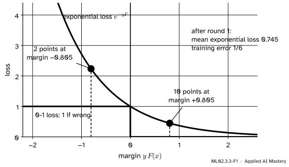
Measure how right the vote is on a point by its margin\({y_i F(x_i)}\): positive when the sign of \(F\) is right, negative when it is wrong, and large when the vote is confident. The exponential loss\({e^{-y F(x)}}\) turns the margin into a cost that is never below the 0-1 loss.
ML02.3.3-F1
The exponential loss lies above the 0-1 loss everywhere. After round 1 the twelve points have margins \(\pm 0.805\); their mean exponential loss, \(0.745\), is an upper bound on the training error \(1/6\).
So pushing the average exponential loss down drags the training error down with it. This lesson shows that AdaBoost is exactly a greedy method for doing that: each round adds one stump, and its \(\alpha_m\) is the step that lowers the average exponential loss the most.
Build it up
Step 1. Add one term at a time.Forward stagewise additive modelling builds \({F_m = F_{m-1} + \beta\, h}\) by choosing a new learner \(h\) and its coefficient \(\beta\) to minimise the training loss, while every earlier term stays frozen. It never goes back to adjust an old stump.
Step 2. Pick the exponential loss. With \({L(y, F) = e^{-yF}}\), the loss of point \(i\) after adding \(\beta h\) factors into two parts:
Step 3. The first factor is a weight. Call it \({\cparam{w_i^{(m)}} = e^{-y_i F_{m-1}(x_i)}}\). It does not depend on \(\beta\) or \(h\), and it is the current loss of point \(i\): large for a point the vote gets wrong, small for one it gets right with confidence. These are AdaBoost’s weights.
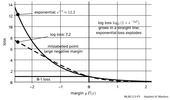
Step 4. Know what the loss rewards. The exponential loss is a smooth stand-in for the 0-1 loss, and so is another one met before. The log loss of logistic regression (ML01.6.2), written for labels \(\pm1\) and scaled to pass through 1 at margin 0, is \({\log_2(1 + e^{-2yF})}\). Far on the wrong side it grows in a straight line, while the exponential loss explodes.
ML02.3.3-F5
A point far on the wrong side, as a mislabelled point often is, costs \({e^{2.5} \approx 12.2}\) under the exponential loss and \(7.2\) under the log loss. AdaBoost’s weight on that point is its exponential loss, so the point dominates every later round.
The formal statement
The stage problem. Summing Step 2 over the points, round \(m\) must solve
The second line adds and subtracts \({e^{-\beta}}\) times the wrong points’ weight.
Choosing \(h\). For any \({\beta > 0}\), the factor \({e^{\beta} - e^{-\beta}}\) is positive, and the first term does not involve \(h\). So the best \(h\) is the one with the smallest weighted error \(\epsilon\): exactly what AdaBoost’s weak learner looks for.
Choosing \(\beta\). Divide by \(\sum_i w_i\), so that the weights sum to 1 and the wrong points hold \(\epsilon\). The stage loss becomes
Since \({g''(\beta)} = (1-\epsilon)e^{-\beta} + \epsilon e^{\beta} > 0\), this is a minimum. It is AdaBoost’s \(\alpha_m\). Putting it back, \({{g(\alpha_m)} = 2\sqrt{\epsilon(1-\epsilon)} = Z_m}\).
The weights follow. The next round’s weights are \({e^{-y_i F_m(x_i)} = w_i^{(m)} e^{-\alpha_m y_i h_m(x_i)}}\): AdaBoost’s update, before rescaling. So AdaBoost is forward stagewise additive modelling with the exponential loss, a fact found by Friedman, Hastie and Tibshirani in 2000, five years after the algorithm itself.
ML02.3.3-F2
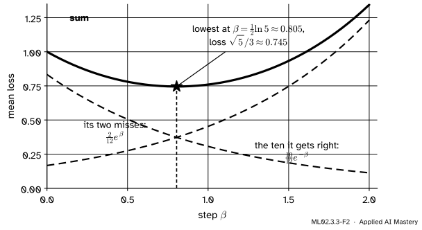
Round 1 on the twelve points. The stage loss is the sum of a falling part (the points the stump gets right) and a rising part (its misses); its lowest point is at \({\beta = \alpha_1}\).
NoteTheorem: the training-error bound
After \(M\) rounds, with \({\gamma_m = \tfrac12 - \epsilon_m}\) the edge of round \(m\), the training error (the fraction of points with \({y_i F_M(x_i) \le 0}\)) satisfies
First,\({I[yF \le 0] \le e^{-yF}}\) for every point: when the margin is at most 0, the exponential is at least 1; otherwise the left side is 0 and the right side is positive. So the training error is at most the mean exponential loss.
Second, the mean exponential loss equals the product of the \(Z_m\). Unrolling the update from \({w_i = 1/n}\), after \(M\) rounds
because each round multiplies by \({e^{-\alpha_m y_i h_m(x_i)}}\) and divides by \(Z_m\), and the exponents add up to \({-y_i F_M(x_i)}\). The final weights sum to 1, so \({\tfrac1n \sum_i e^{-y_i F_M(x_i)} = Z_1 \cdots Z_M}\).
Third, each \(Z_m\) is small when the edge is large. With \({\epsilon = \tfrac12 - \gamma}\),
using \({1 + x \le e^x}\) with \({x = -4\gamma^2}\). Multiplying over the rounds turns the sum in the exponent into \(\sum_m \gamma_m^2\). \(\square\)
What it promises. If every round has an edge of at least \({\gamma > 0}\), the training error is at most \({e^{-2M\gamma^2}}\), which falls exponentially in \(M\). A training error below \(1/n\) means no mistakes at all, so after \({M > \ln n / (2\gamma^2)}\) rounds the vote fits the training data perfectly.
Go deeper: what does the exponential loss estimate?
Fix an input \(x\) and let \({p = \Prob(Y = 1 \mid x)}\). The expected exponential loss of a score \(F\) at \(x\) is \({p\, e^{-F} + (1-p)\, e^{F}}\). Its derivative in \(F\) is \({-p e^{-F} + (1-p) e^{F}}\), which is zero when \({e^{2F} = p/(1-p)}\):
\[
F^*(x) = \frac12 \ln \frac{p}{1-p} .
\]
So AdaBoost’s score estimates half the log-odds, and \({p = 1/(1 + e^{-2F})}\). The log loss written for labels \(\pm 1\) with the score \(2F\), \({\ln(1 + e^{-2yF})}\), has the same minimiser, which is why the two losses are compared with that factor of 2. They agree on the whole population but not on a finite, noisy sample.
Worked example
Round 1 as a stage problem. With equal weights, the stump \({x_1 \le 3.5}\) gets ten points right and two wrong, so the mean stage loss is
Their product simplifies neatly: the numerators give \({2\sqrt{5 \cdot 6 \cdot 15} = 2\sqrt{450}}\), which is \(30\sqrt2\), over \({3 \cdot 5 \cdot 4 = 60}\), so
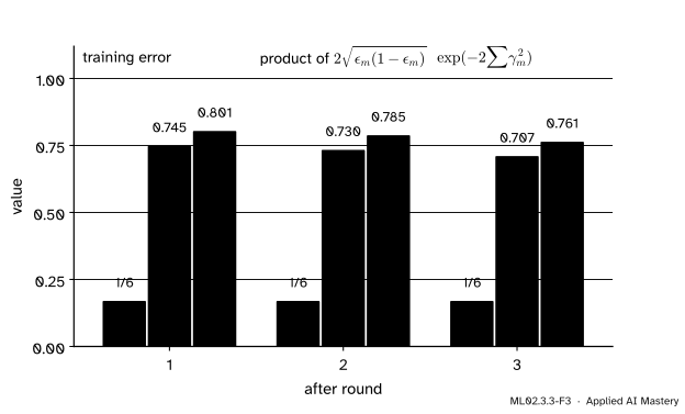
The edges are \({\gamma = \tfrac13, \tfrac{1}{10}, \tfrac18}\), so \(\sum \gamma_m^2 = \tfrac19 + \tfrac{1}{100} + \tfrac{1}{64} \approx 0.137\) and the looser bound is \({e^{-0.273} \approx 0.761}\). The chain reads \({1/6 \le 0.707 \le 0.761}\).
ML02.3.3-F3
The two bounds fall round by round and always sit above the training error. Here the error stays at \(1/6\); the next sections ask why.
Code
Forward stagewise modelling done by brute force: for every stump, find the best step \(\beta\) with a one-dimensional minimiser, and keep the pair with the lowest mean exponential loss. Nothing in this code mentions AdaBoost’s formulas.
import numpy as npfrom scipy.optimize import minimize_scalarX = np.array([(1, 1), (2, 1), (1, 2), (2, 3), (3, 2), (5, 5), (4, 1), (5, 2), (5, 3), (4, 4), (2, 5), (6, 5)], dtype=float)y = np.array([-1] *6+ [1] *6)stumps = [(j, t, s) for j in (0, 1)for t in (np.unique(X[:, j])[:-1] + np.unique(X[:, j])[1:]) /2for s in (1, -1)]predict =lambda j, t, s: np.where(X[:, j] > t, s, -s)F = np.zeros(12)for m inrange(1, 4): best =Nonefor j, t, s in stumps: h = predict(j, t, s) res = minimize_scalar(lambda b: np.mean(np.exp(-y * (F + b * h))), bounds=(0, 5), method="bounded", options={"xatol": 1e-10})if best isNoneor res.fun < best[0] -1e-9: best = (res.fun, res.x, (j, float(t), s), h) loss, beta, stump, h = best F = F + beta * hprint(f"stage {m}: stump {stump}, beta = {beta:.4f}, mean exp loss = {loss:.4f}")print("training error:", np.mean(y * F <=0))
stage 1: stump (0, 3.5, 1), beta = 0.8047, mean exp loss = 0.7454
stage 2: stump (0, 1.5, 1), beta = 0.2027, mean exp loss = 0.7303
stage 3: stump (0, 5.5, 1), beta = 0.2554, mean exp loss = 0.7071
training error: 0.16666666666666666
The steps are AdaBoost’s \(\alpha_m\) and the losses are the products of the \(Z_m\). Now the two bounds from the formulas:
eps = np.array([1/6, 2/5, 3/8])Z =2* np.sqrt(eps * (1- eps))gamma =0.5- epsprint("Z:", np.round(Z, 4), " product:", round(Z.prod(), 4))print("exp(-2 sum gamma^2):", round(np.exp(-2* np.sum(gamma**2)), 4))print("rounds needed for zero error with n = 100 and gamma = 0.1:",int(np.floor(np.log(100) / (2*0.1**2))) +1)
Z: [0.7454 0.9798 0.9682]  product: 0.7071
exp(-2 sum gamma^2): 0.7607
rounds needed for zero error with n = 100 and gamma = 0.1: 231
Explore
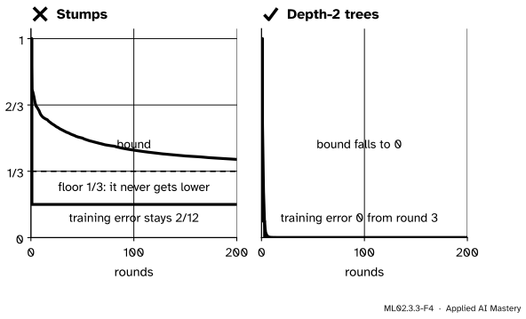
The AdaBoost stepper in ML02.3.2 plots the training error beside the bound \(Z_1 \cdots Z_m\) round by round. With stumps on the twelve points the bound falls slowly and the error never moves from \(2/12\). The picture below explains why.
ML02.3.3-F6
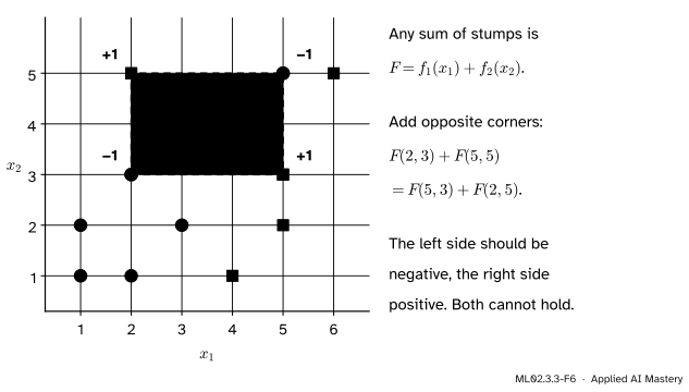
Four of the twelve points form an XOR pattern on a rectangle. A sum of stumps adds a function of \(x_1\) to a function of \(x_2\), and such a sum takes equal totals on the two diagonals.
Each opposite-corner sum contains \({f_1(2) + f_1(5) + f_2(3) + f_2(5)}\), so the two totals are equal. In margins: the four corner margins add up to zero. So at least one of them is at most zero, and the training error of any sum of stumps is at least \(1/12\). More: since \({e^{-m}}\) is convex, four margins with sum zero have \({\sum e^{-m_k} \ge 4 e^{0} = 4}\), so the mean exponential loss can never fall below \({4/12 = 1/3}\). The bound of the theorem then forces \({\exp(-2\sum\gamma_m^2) \ge \tfrac13}\): the edges must shrink towards zero. Depth-2 trees can represent the XOR, and with them the error reaches 0 in round 3.
Pitfalls
ML02.3.3-F4
Wrong beside right. The bound reaches zero only while each learner keeps an edge. With stumps on the twelve points it stalls above \(1/3\); with depth-2 trees it does not.
“AdaBoost always drives the training error to zero.”
Only under the weak learning condition: an edge \({\gamma > 0}\) in every round. If the weak learners cannot represent the pattern, as stumps cannot represent the XOR of the four corner points, the edges shrink, the bound stalls and the training error stops falling.
“AdaBoost minimises the training error.”
It minimises the exponential loss, one stump at a time. The training error can sit still while the exponential loss keeps falling, as on the twelve points with stumps, and the loss goes on falling even after the training error reaches zero, because the margins keep growing.
“Exponential loss and log loss have the same minimiser, so AdaBoost is as robust as logistic regression.”
They agree on the whole population, not on a finite sample. A mislabelled point sits at a large negative margin, where the exponential loss, and with it the point’s weight, grows without limit, while the log loss grows only in a straight line. Lesson ML02.3.4 measures the damage.
Check yourself
Recall
1. What is forward stagewise additive modelling?
Show answer
Building \({F_m = F_{m-1} + \beta h}\) one term at a time, choosing each new \(h\) and \(\beta\) to minimise the loss while every earlier term stays fixed.
2. With the exponential loss, what are the weights \(w_i^{(m)}\)?
Show answer
\({w_i^{(m)} = e^{-y_i F_{m-1}(x_i)}}\): the current exponential loss of each point.
3. Why does minimising the stage loss over \(h\) mean minimising weighted error?
Show answer
The stage loss is \({e^{-\beta} \sum_i w_i + (e^{\beta} - e^{-\beta})}\) times the weighted error, and \({e^{\beta} - e^{-\beta} > 0}\) for \({\beta > 0}\).
4. State the training-error bound.
Show answer
Training error \(\le \prod_m 2\sqrt{\epsilon_m(1-\epsilon_m)} \le \exp(-2\sum_m \gamma_m^2)\), with \({\gamma_m = \tfrac12 - \epsilon_m}\).
5. What is the product \(Z_1 Z_2 Z_3\) on the twelve points?
1.★ A stump gets three quarters of the weight right. Write its stage loss \(g(\beta)\), find the best \(\beta\) by calculus, and find \({g(\beta)}\) there.
Show solution
\({g(\beta) = \tfrac34 e^{-\beta} + \tfrac14 e^{\beta}}\). Then \({{g'(\beta)} = 0}\) gives \({e^{2\beta} = 3}\), so \({\beta = \tfrac12 \ln 3 \approx 0.549}\). There \({e^{-\beta} = 1/\sqrt3}\) and \({e^{\beta} = \sqrt3}\), so \(g = \tfrac{3}{4\sqrt3} + \tfrac{\sqrt3}{4} = \tfrac{\sqrt3}{2} \approx 0.866\), which is \(2\sqrt{\tfrac14 \cdot \tfrac34}\).
2.★★ Every round of a run has edge at least \({\gamma = 0.1}\) on \({n = 100}\) training points. After how many rounds does the theorem guarantee zero training error?
Show solution
The error is at most \({e^{-2M(0.1)^2} = e^{-0.02M}}\). Zero errors are guaranteed once this is below \(1/100\), that is, \({0.02M > \ln 100 \approx 4.605}\), so \({M > 230.3}\). After 231 rounds the training error must be 0.
3.★★★ Four numbers \(m_1, \dots, m_4\) add up to zero. Show that \({\sum_k e^{-m_k} \ge 4}\), and conclude that a sum of stumps has mean exponential loss at least \(1/3\) on the twelve points.
Show solution
The function \({e^{-m}}\) is convex, so its average over four points is at least its value at their average (Jensen’s inequality):
So \({\sum_k e^{-m_k} \ge 4}\). For a sum of stumps, the margins at \((2,3)\), \((5,5)\), \((5,3)\) and \((2,5)\) are \({-F(2,3)}\), \({-F(5,5)}\), \(F(5,3)\) and \(F(2,5)\), and they add to zero because the two diagonal sums of \(F\) are equal. The other eight points add non-negative losses, so the mean over all twelve is at least \({4/12 = 1/3}\).
Summary card
AdaBoost greedily minimises the mean exponential loss, which bounds the training error.
Weak spot. A badly wrong point’s weight grows like \({e^{-yF}}\).
Sources and next steps
Sources. Each was opened and checked against this lesson on 15 November 2026.
Trevor Hastie, Robert Tibshirani and Jerome Friedman, The Elements of Statistical Learning, 2nd edition. Algorithm 10.2 and section 10.3 (forward stagewise additive modelling); section 10.4, equations (10.8) to (10.15), the derivation of AdaBoost from the exponential loss, with \(\beta_m\) in (10.12); section 10.5, equation (10.16), the half log-odds, credited to Friedman et al. (2000); section 10.6 and Figure 10.4, the losses against the margin, the binomial deviance \({\log(1 + e^{-2yf})}\), and AdaBoost’s degradation under mislabelled training data.
Robert E. Schapire, The Boosting Approach to Machine Learning: An Overview, Springer, 2003. Section 3, equations (2) to (5): the training error is at most the mean exponential loss, which equals \(\prod_t Z_t\); with binary learners \(Z_t = 2\sqrt{\epsilon_t(1-\epsilon_t)} = \sqrt{1 - 4\gamma_t^2} \le e^{-2\gamma_t^2}\).
Robert E. Schapire, Explaining AdaBoost. Section 2 states the weak learning condition \({\epsilon_t \le \tfrac12 - \gamma}\); section 4 describes AdaBoost as minimising the exponential loss by coordinate descent; section 6 reports its susceptibility to noise.
Kilian Weinberger, Cornell CS4780, lecture 19: Boosting. Derives the step size by setting the derivative of the exponential loss to zero, and shows the training loss falling exponentially.
Next.ML02.3.4 AdaBoost in practice runs AdaBoost on real data and flips labels on purpose. ML02.4 replaces the exponential loss by any differentiable loss: gradient boosting.