Any method written in dot products can be kernelised. Rewrite ridge regression with one weight per example, fit kernel ridge regression on the eight-point set, count what an exact kernel method costs, and cut that cost with random Fourier features and the Nystroem method.
ML02.8.4L2 Intermediate30 minIn review (what this means)
The maths and code on this page are checked by automated tests on every change, but an independent reader has not signed it off yet. Spot a mistake or a confusing step? Tell us.
Prove the identity (X’X + lambda I)^-1 X’ = X’(XX’ + lambda I)^-1 and use it to write ridge regression with one weight per example.
Derive kernel ridge regression and fit it from scratch on the eight-point set, matching scikit-learn’s KernelRidge.
Count the memory and time an exact kernel method needs as the number of examples grows.
Explain random Fourier features and the Nystroem method, and use them with a linear model on load_digits.
The question
The kernel trick made the SVM bend. But nothing in the trick was about margins: it only needed an algorithm that touches the data through dot products. Ridge regression (ML01.9.1) solves for one weight per feature. Can it be rewritten with one weight per example, so that a kernel can take over? And what does that cost when there are a million examples?
From the last lesson
1. How does a kernel SVM score a new point?
Show answer
\({f(\vect{x}) = \sum_i \alpha_i y_i\, k(\vect{x}_i, \vect{x}) + b}\), a weighted sum of kernel values with the support vectors.
2. How were \(\gamma\) and \(C\) chosen for the moons?
Show answer
By five-fold cross-validation over a grid spaced by factors of 10 (GridSearchCV), which picked \({C = 1}\) and \({\gamma = 10}\).
Intuition
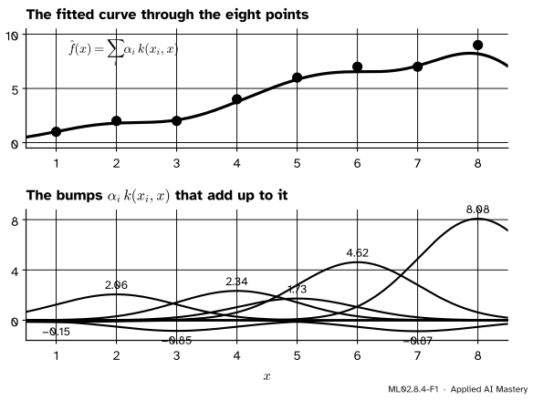
Here is what the answer looks like on the course’s eight-point regression set, \({x = 1, \dots, 8}\) with \({y = (1, 2, 2, 4, 6, 7, 7, 9)}\). Kernel ridge regression puts an RBF bump on every training point, gives each bump a weight \({\alpha_i}\), and adds them up.
ML02.8.4-F1
Top: the fitted curve. Bottom: the eight bumps it is made of, one per training point, each scaled by its weight. Adding the bottom curves gives the top one. Here \(\gamma = 0.5\) and \(\lambda = 0.1\).
The weights are not the features’ weights of ordinary ridge. They belong to the examples, as the SVM’s \({\alpha_i}\) did. Some are negative: the bump at \(x = 3\) pulls the curve down so that it passes near the point \((3, 2)\) between its rising neighbours. This lesson shows that ridge regression can always be written this way, and then that the RBF kernel can replace the dot product.
Build it up
Step 1. Ridge, in this lesson’s convention. For a table \(\mat{X}\) with one example per row and targets \(\vect{y}\), with no bias for now, ridge minimises the sum of squared errors plus a price on the weights:
This is the convention of scikit-learn’s Ridge and KernelRidge. ML01.9.1 used the mean of the squared errors instead, so its \(\lambda\) is ours divided by \(n\).
Step 2. Its solution. The gradient is \({-2\mat{X}\T(\vect{y} - \mat{X}\vect{w}) + 2\lambda\vect{w}}\). Setting it to zero and collecting the terms in \(\vect{w}\) gives
The matrix to invert is \(d \times d\), one row per feature.
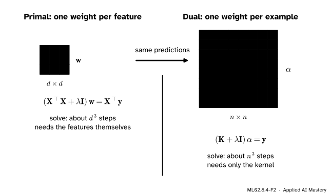
Step 3. Turn it inside out. The identity proved below moves the inverse to the other side: \({\vect{w} = \mat{X}\T(\mat{X}\mat{X}\T + \lambda\mat{I})^{-1}\vect{y}}\). Now the matrix to invert is \(n \times n\), one row per example, and its entries \({(\mat{X}\mat{X}\T)_{ij} = \vect{x}_i \cdot \vect{x}_j}\) are dot products: the Gram matrix of the plain dot product.
ML02.8.4-F2
Two systems for one ridge fit. The primal has one unknown per feature and needs the features. The dual has one unknown per example and needs only dot products, so a kernel can stand in for them.
Step 4. Predict with dot products. Write \({\vect{\alpha} = (\mat{X}\mat{X}\T + \lambda\mat{I})^{-1}\vect{y}}\). Then \({\vect{w} = \mat{X}\T\vect{\alpha} = \sum_i \alpha_i \vect{x}_i}\), and the prediction at a new point is \({\vect{w} \cdot \vect{x} = \sum_i \alpha_i\, \vect{x}_i \cdot \vect{x}}\). Both the fit and the prediction now touch the data only through dot products.
Step 5. Swap in a kernel. Replace every dot product by \({k(\vect{x}_i, \vect{x}_j)}\). That is kernel ridge regression, and it is ridge regression in the kernel’s lifted space.
The formal statement
NoteResult: the push-through identity
For any \(n \times d\) matrix \(\mat{X}\) and any \({\lambda > 0}\),
Proof. Both brackets can be inverted. For any \({\vect{v} \ne \vect{0}}\), \({\vect{v}\T(\mat{X}\T\mat{X} + \lambda\mat{I})\vect{v}} = {\norm{\mat{X}\vect{v}}^2} + {\lambda\norm{\vect{v}}^2} > 0\), so the matrix sends no non-zero vector to \(\vect{0}\); the same argument with \(\mat{X}\T\) in place of \(\mat{X}\) covers the other. Now multiply out \({\mat{X}\T}\) times the second bracket, in two ways:
Multiply both ends on the left by \({(\mat{X}\T\mat{X} + \lambda\mat{I})^{-1}}\) and on the right by \({(\mat{X}\mat{X}\T + \lambda\mat{I})^{-1}}\). On the left end the second inverse cancels its bracket, and on the right end the first inverse cancels its bracket, leaving \({\mat{X}\T(\mat{X}\mat{X}\T + \lambda\mat{I})^{-1}} = {(\mat{X}\T\mat{X} + \lambda\mat{I})^{-1}\mat{X}\T}\).
NoteKernel ridge regression
With a kernel \(k\), its Gram matrix \(\mat{K}\) on the training inputs and a price \({\lambda > 0}\),
It is ridge regression, with the loss of Step 1, on the lifted features \({\varphi(\vect{x})}\).
One more fact falls out. Rearrange \({(\mat{K} + \lambda\mat{I})\vect{\alpha} = \vect{y}}\) as \({\lambda\vect{\alpha} = \vect{y} - \mat{K}\vect{\alpha}}\). The \(i\)-th entry of \({\mat{K}\vect{\alpha}}\) is \({\hat{f}(\vect{x}_i)}\), so
each example’s weight is its residual divided by the price. Unlike the SVM, kernel ridge gives almost every example a non-zero weight, so it keeps all \(n\) of them.
The cost of being exact. An exact kernel method stores \(\mat{K}\), which has \(n^2\) entries, and solves an \(n \times n\) system, which takes a number of steps that grows like \(n^3\). At 8 bytes a number, the 1,437 training images of load_digits need 16.5 MB; 100,000 examples would need 80 GB. Doubling \(n\) multiplies the memory by 4 and the solving time by about 8.
Two remedies. Both trade the exact kernel for an explicit map with \(D\) coordinates, then fit a plain linear model on it, whose cost grows only in step with \(n\).
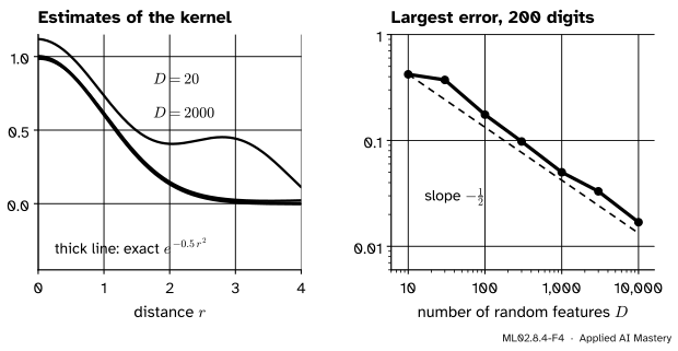
Random Fourier features (Rahimi and Recht, 2007). For the RBF kernel, draw \(D\) random directions \({\vect{\omega}_j}\) from a normal distribution with variance \({2\gamma}\) in each coordinate and \(D\) random shifts \(b_j\) between 0 and \({2\pi}\), and map \({z_j(\vect{x}) = \sqrt{2/D}\,\cos(\vect{\omega}_j \cdot \vect{x} + b_j)}\). Then \({\vect{z}(\vect{x}) \cdot \vect{z}(\vect{x}')}\) is an average of \(D\) random terms whose mean is exactly \({k(\vect{x}, \vect{x}')}\), so its error shrinks like \({1/\sqrt{D}}\). scikit-learn’s RBFSampler builds this map.
The Nyström method (Williams and Seeger). Choose \(m\) of the training points as landmarks and approximate the Gram matrix by \({\mat{K}_{nm} \mat{K}_{mm}^{-1} \mat{K}_{mn}}\), where \({\mat{K}_{nm}}\) holds the kernel between every point and every landmark. This is exact on the landmarks and costs about \({m^2 n}\) steps. scikit-learn’s Nystroem builds the matching map with \(m\) coordinates.
Go deeper: why random cosines average to the RBF kernel
Write \({\vect{\delta} = \vect{x} - \vect{x}'}\) and take one random direction \(\vect{\omega}\) and shift \(b\). Call the two angles \({A = \vect{\omega} \cdot \vect{x} + b}\) and \({B = \vect{\omega} \cdot \vect{x}' + b}\). The product rule gives
\[
\begin{aligned}
2\cos A \cos B &= \cos(A - B) \\
&\quad + \cos(A + B),
\end{aligned}
\]
where \({A - B = \vect{\omega} \cdot \vect{\delta}}\) and \({A + B = \vect{\omega} \cdot (\vect{x} + \vect{x}') + 2b}\).
With \(b\) uniform on \({[0, 2\pi]}\), the angle in the last term is uniform round the circle too, so that term averages to 0. For the first, a normal \(\vect{\omega}\) with variance \({2\gamma}\) in each coordinate makes \({\vect{\omega} \cdot \vect{\delta}}\) a normal number with mean 0 and variance \({s^2 = 2\gamma\norm{\vect{\delta}}^2}\), and the average of \(\cos\) of a normal number with mean 0 and variance \(s^2\) is \({e^{-s^2/2}}\). So the mean of the product is \({e^{-\gamma\norm{\vect{\delta}}^2}}\), the RBF kernel. The factor \({\sqrt{2/D}}\) in each coordinate turns the dot product of two \(D\)-vectors into the average of \(D\) such products.
ML02.8.4-F4
Left: random Fourier features estimate the RBF kernel; with 2,000 features the estimate is hard to tell from the truth. Right: the largest error over a \(200 \times 200\) Gram matrix falls like \({1/\sqrt{D}}\).
Worked example
Ridge through the origin on the eight points, \(\lambda = 4\), by both routes.
With one feature and the plain dot product, \({\mat{X}\T\mat{X} = \sum_i x_i^2}\) and \({\mat{X}\T\vect{y} = \sum_i x_i y_i}\).
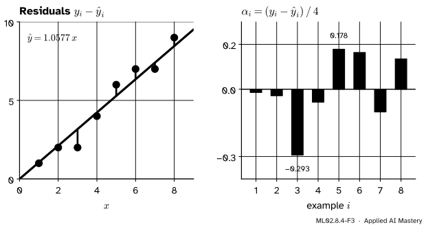
Dual. The weights are the residuals divided by 4. At \({x = 3}\) the line predicts \({3 \times 1.0577 = 3.173}\), so \({\alpha_3 = (2 - 3.173)/4 = -0.293}\). At \({x = 8}\) it predicts \({8.462}\), so \({\alpha_8 = (9 - 8.462)/4 = 0.135}\). All eight are in the figure. Rebuild the weight from them:
The third line uses \({220 \times 52} - {55 \times 204} = {11{,}440 - 11{,}220} = 220\) over \({4 \times 52 = 208}\). Both routes give the same line.
ML02.8.4-F3
The dual weights are the residuals, divided by \(\lambda = 4\). The point \((3, 2)\) sits furthest below the line and gets the most negative weight.
Now the RBF kernel with \({\gamma = 0.5}\) and \({\lambda = 0.1}\): the code below builds the \(8 \times 8\) Gram matrix and solves for the weights of the opening figure. The prediction at \({x = 4.5}\) is 4.88, between the neighbours at 4 and 6.
Code
Kernel ridge from scratch, checked against the primal for the linear kernel and against KernelRidge for the RBF kernel.
import numpy as npfrom sklearn.kernel_ridge import KernelRidgex = np.arange(1, 9, dtype=float)y = np.array([1, 2, 2, 4, 6, 7, 7, 9], dtype=float)def kernel_ridge(K, y, lam):return np.linalg.solve(K + lam * np.eye(len(y)), y)alpha_lin = kernel_ridge(np.outer(x, x), y, 4.0)w = (x @ y) / (x @ x +4.0)print("primal w =", round(w, 4), " dual: sum alpha_i x_i =", round(alpha_lin @ x, 4))print("dual weights:", np.round(alpha_lin, 4))rbf =lambda a, b, g=0.5: np.exp(-g * (a[:, None] - b[None, :]) **2)alpha = kernel_ridge(rbf(x, x), y, 0.1)predict =lambda q: rbf(np.atleast_1d(q), x) @ alphalibrary = KernelRidge(alpha=0.1, kernel="rbf", gamma=0.5).fit(x.reshape(-1, 1), y)print("RBF weights:", np.round(alpha, 3))print("prediction at 4.5:", np.round(predict(4.5), 3), " KernelRidge:", np.round(library.predict([[4.5]]), 3))print("residuals / lambda = weights:", np.allclose((y - predict(x)) /0.1, alpha))print("far from the data, x = 10 and 12:", np.round(predict(np.array([10.0, 12.0])), 3))
primal w = 1.0577    dual: sum alpha_i x_i = 1.0577
dual weights: [-0.0144 -0.0288 -0.2933 -0.0577  0.1779  0.1635 -0.101   0.1346]
RBF weights: [-0.146  2.059 -0.846  2.336  1.73   4.617 -0.872  8.076]
prediction at 4.5: [4.881]  KernelRidge: [4.881]
residuals / lambda = weights: True
far from the data, x = 10 and 12: [1.085 0.003]
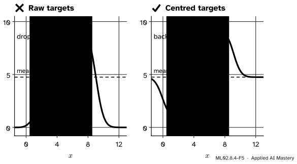
KernelRidge has no intercept, and far from the data every bump has died away, so the prediction sinks to 0: 1.085 at \({x = 10}\) and 0.003 at \({x = 12}\). The pitfalls return to this.
Next, the cost. On the 1,437 training images of load_digits (64 pixels each, ten classes), fit the exact kernel ridge with one-hot targets, and two approximations followed by a linear ridge classifier. The times print on your machine; the accuracies are what to compare.
exact kernel ridge         test accuracy 0.989   0.044 s
Nystroem, m = 300          test accuracy 0.986   0.021 s
random features, D = 1000  test accuracy 0.992   0.036 s
Gram matrix of the training set: 16.5 MB
All three reach about 99% on the 360 test images. At this size the exact method is quick, so the approximations buy nothing yet. Their value shows when \(n\) grows: the exact fit’s memory grows like \(n^2\) and its time like \(n^3\), while each approximation’s cost grows in step with \(n\).
Explore
This module’s interactive, the kernel lift, lives in lesson 3. Its RBF mode shows the same bumps as this lesson’s opening figure, used for classification: watch them merge or separate as \(\gamma\) changes.
Pitfalls
ML02.8.4-F5
Wrong beside right. Left: with no intercept, the fit returns to 0 wherever the bumps run out. Right: subtract the mean of \(y\) before fitting and add it back after, and the fit returns to the mean instead.
“Kernel ridge fits an intercept, like Ridge does.”
KernelRidge has no intercept: the prediction is \({\sum_i \alpha_i k(\vect{x}_i, \vect{x})}\) and nothing else. With an RBF kernel it sinks to 0 away from the data, 0.003 at \({x = 12}\) on the eight points. Centre the targets first: the same fit on \({y - 4.75}\), with 4.75 added back, predicts 4.752 at \({x = 12}\), and its training error falls from 0.126 to 0.068.
“A price \(\lambda\) from ML01.9 can be used as alpha here.”
ML01.9 charged the price against the mean squared error; Ridge and KernelRidge charge it against the sum. The same fit needs alpha set to \({n\lambda}\). Always check which loss a library’s parameter belongs to.
“A kernel method works for any amount of data.”
The exact method stores \(n^2\) numbers and solves in about \(n^3\) steps: 80 GB of memory for 100,000 examples. Beyond some tens of thousands, use an approximation or a model that scales better, and, as scikit-learn’s guide advises, compare it with the exact method on a sample where you can.
3. How is each dual weight related to its example’s residual?
Show answer
\({\alpha_i = (y_i - \hat{f}(\vect{x}_i)) / \lambda}\): the residual divided by the price.
4. How do the memory and the time of an exact kernel method grow with \(n\)?
Show answer
Memory like \(n^2\), for the Gram matrix; time like \(n^3\), for solving the \(n \times n\) system.
5. What do random Fourier features and the Nyström method each build?
Show answer
Both build an explicit map with a fixed number of coordinates, on which a linear model is fitted. Random Fourier features use \(D\) random cosines whose dot products average to the RBF kernel; the Nyström method uses the kernel with \(m\) landmark points, approximating \(\mat{K}\) by \({\mat{K}_{nm}\mat{K}_{mm}^{-1}\mat{K}_{mn}}\).
Exercises
1.★ Fit kernel ridge by hand to the two points \((4, 4)\) and \((5, 6)\) with the RBF kernel, \({\gamma = 0.5}\) and \({\lambda = 0.1}\), and predict at \({x = 4.5}\).
Show solution
The kernel between the two points is \({e^{-0.5} = 0.6065}\), so
At \({x = 4.5}\) both kernels are \({e^{-0.125} = 0.8825}\), so the prediction is \({0.8825 \times (0.903 + 4.956) = 5.17}\).
2.★★ An exact kernel ridge fit on 10,000 examples takes 20 seconds and its Gram matrix fills 800 MB. Estimate both for 40,000 examples. How many numbers does a Nyström map with \(m = 500\) landmarks store for the 40,000 examples?
Show solution
Four times the examples: the memory grows by \({4^2 = 16}\), to 12.8 GB, and the time by about \({4^3 = 64}\), to about 1,280 seconds, over 21 minutes. The Nyström map stores \({40{,}000 \times 500 = 20}\) million numbers, 160 MB at 8 bytes each, and its cost grows only in step with \(n\).
3.★★★ Prove that \({\alpha_i = (y_i - \hat{f}(\vect{x}_i))/\lambda}\). Then suppose \(\mat{K}\) can be inverted and let \(\lambda\) shrink towards 0. What happens to the residuals, and what does that say about overfitting?
Show solution
From \({(\mat{K} + \lambda\mat{I})\vect{\alpha} = \vect{y}}\), move \({\mat{K}\vect{\alpha}}\) across: \({\lambda\vect{\alpha} = \vect{y} - \mat{K}\vect{\alpha}}\). The \(i\)-th entry of \({\mat{K}\vect{\alpha}}\) is \({\sum_j \alpha_j k(\vect{x}_j, \vect{x}_i) = \hat{f}(\vect{x}_i)}\); divide by \(\lambda\).
As \({\lambda \to 0}\) with \(\mat{K}\) invertible, \({\vect{\alpha} \to \mat{K}^{-1}\vect{y}}\), a fixed vector. The residuals are \({\lambda\vect{\alpha}}\), so they shrink to 0: the fit passes through every training point. For the RBF kernel, whose Gram matrix on distinct points can always be inverted, an unpenalised fit interpolates the noise as well as the signal. The price \(\lambda\) is what stops kernel ridge from overfitting.
Summary card
Write a method in dot products, and a kernel can take over.
Kernel ridge.\({\vect{\alpha} = (\mat{K} + \lambda\mat{I})^{-1}\vect{y}}\), \({\hat{f}(\vect{x}) = \sum_i \alpha_i k(\vect{x}_i, \vect{x})}\); no intercept, so centre \(y\).
Cost.\(n^2\) memory and about \(n^3\) time.
Remedies. Random Fourier features (RBFSampler) and Nyström (Nystroem), then a linear model.
Frontier note: where kernels lead
Kernel ridge regression’s prediction is exactly the mean prediction of a zero-mean Gaussian process with the same kernel and a noise variance of \(\lambda\) (Rasmussen and Williams, section 6.2.2), which module ML05.8 builds from the Bayesian side, with error bars. Why the RBF kernel’s infinite lift behaves so well is the theory of reproducing kernel Hilbert spaces, in ML06.8 and M11.5.
Sources and next steps
Sources. Each was opened and checked against this lesson on 15 November 2026.
Tengyu Ma and Andrew Ng, CS229 Lecture Notes, Stanford University, Section 5.3. Rewrites gradient descent for least squares with one coefficient \({\beta_i}\) per example, stores the kernel values in advance, and predicts with \({\sum_i \beta_i K(x^{(i)}, x)}\) (equation 5.12).
Kilian Weinberger, Lecture 14: Kernels continued, Cornell CS4780 (Fall 2018). Gives kernelised least squares as \({\vect{\alpha} = \mat{K}^{-1}\vect{y}}\) and kernel ridge regression as \({\vect{\alpha} = (\mat{K} + \tau^2\mat{I})^{-1}\vect{y}}\).
scikit-learn 1.9 User Guide, Section 1.3, Kernel ridge regression, and the API reference for KernelRidge. The guide says KRR combines ridge regression with the kernel trick, can be fitted in closed form, and learns a model that is not sparse. The reference describes alpha as the regularisation strength and dual_coef_ as the weight vector in kernel space; the class has no intercept.
scikit-learn 1.9 User Guide, Section 8.7, Kernel approximation. Describes Nystroem as subsampling rows and columns of the kernel matrix, with cost \({O(n_{\text{components}}^2\, n)}\) against \({O(n^3)}\) for the exact method, and RBFSampler as a Monte Carlo approximation of the RBF kernel after Rahimi and Recht, and advises comparing approximate embeddings with exact kernel methods when possible.
Ali Rahimi and Ben Recht, Random Features for Large-Scale Kernel Machines, NeurIPS 2007, Section 3. Defines \({z_\omega(\vect{x}) = \sqrt{2}\cos(\omega\T\vect{x} + b)}\) with \(\omega\) drawn from the kernel’s Fourier transform and \(b\) uniform on \({[0, 2\pi]}\), averages \(D\) of them with the factor \({1/\sqrt{D}}\), and bounds the error with Hoeffding’s inequality.
Christopher Williams and Matthias Seeger, Using the Nyström Method to Speed Up Kernel Machines, Advances in Neural Information Processing Systems 13. Approximates the Gram matrix by \({\tilde{\mat{K}} = \mat{K}_{n,m}\mat{K}_{m,m}^{-1}\mat{K}_{m,n}}\) (equation 10) from \(m\) sampled columns, at a cost of \({O(m^2 n)}\) instead of \({O(n^3)}\).
Carl Edward Rasmussen and Christopher Williams, Gaussian Processes for Machine Learning, MIT Press, 2006, Section 6.2.2. Minimises a squared-error loss plus the kernel norm, finds the weights \({(\mat{K} + \sigma_n^2\mat{I})^{-1}\vect{y}}\), and notes that the prediction is exactly the Gaussian process’s predictive mean.
Next. Module ML02.9, Discriminant analysis, returns to classification with a generative model built from Gaussian clouds.