Treat a message as a bag of word counts and each class as a die with one face per word. Estimate the faces by smoothed counting, work a tiny corpus by hand, and discover that naive Bayes is a linear classifier whose weights are log ratios of word probabilities.
ML02.6.3L2 Intermediate25 minIn review (what this means)
The maths and code on this page are checked by automated tests on every change, but an independent reader has not signed it off yet. Spot a mistake or a confusing step? Tell us.
Represent a document as a bag of word counts and write the multinomial likelihood of a class.
Derive the maximum-likelihood word probabilities as relative frequencies, and smooth them with pseudo-counts.
Show that the log posterior is linear in the counts, and read each word’s weight as a log ratio of its probabilities.
Train multinomial naive Bayes by hand, from scratch and with CountVectorizer and MultinomialNB.
The question
Two messages: “free lunch” and “free free lunch”. The Bernoulli model of the last lesson sees the same two words in both and gives them the same answer. Surely shouting “free” twice says something? And when you write out what naive Bayes computes on a text, what kind of classifier turns out to be hiding inside it?
From the last lesson
1. For \(d\) binary features, how many probabilities per class does naive Bayes estimate, and how many would the full table need?
Show answer
\(d\) for naive Bayes, and \({2^d - 1}\) for the full table.
2. Why does a naive Bayes implementation add logs instead of multiplying probabilities?
Show answer
A product of hundreds of small probabilities underflows to 0.0. The sum of the logs is an ordinary number and ranks the classes the same way.
Intuition
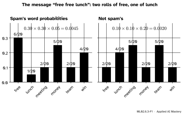
Forget the order of the words and keep only how often each one appears: this is a bag of words. Now imagine each class as a die with one face per word in the vocabulary, loaded differently for each class. A spam message is made by rolling the spam die once per word. To classify a message, ask which die would more likely have rolled it.
ML02.6.3-F1
Each class as a loaded die. The message “free free lunch” is two rolls of “free” and one of “lunch”. The spam die makes it \({0.0045/0.0020 = 2.25}\) times as likely as the other die does.
“Free” is three times as likely on the spam die and appears twice, so it counts twice. “Lunch” is four times as likely on the other die and appears once. With equal priors the odds of spam are \({3 \times 3 \times \tfrac14 = 2.25}\), a probability of \({2.25/3.25 = 9/13}\).
Build it up
Step 1. A message becomes a count vector. Fix a vocabulary of \(V\) words. A message becomes \({\vect{x} = (x_1, \dots, x_V)}\), where \(x_j\) counts the appearances of word \(j\). “Free free lunch” over the vocabulary (free, lunch, meeting, money, team, win) is \({(2, 1, 0, 0, 0, 0)}\).
Step 2. A tiny corpus. Eight short messages, four of each class:
Spam (class 1)
Not spam (class 0)
free money free win
team meeting lunch
win free money
meeting team lunch free
free money team
team lunch meeting
win free money meeting
win money meeting team
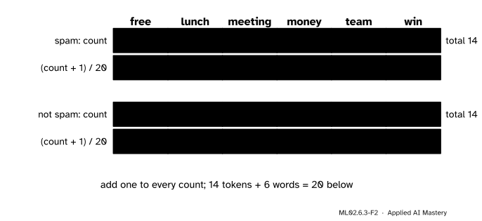
Step 3. Count each class’s words. Add the count vectors of each class. Each class happens to have 14 words in all.
ML02.6.3-F2
Training is counting. Each word probability is its count plus one, over the class total plus the vocabulary size.
Step 4. Smoothed relative frequencies. The probability of word \(j\) on the die of class \(k\) is its share of the class’s words. “Lunch” never appears in spam, so add one pseudo-count to every word first. With six words, that adds six to the total: \({\hat\theta_{1,\text{free}} = (5 + 1)/(14 + 6) = 6/20}\).
The formal statement
NoteDefinition: multinomial naive Bayes
Each class \(k\) has a prior \(\pi_k\) and word probabilities \({\theta_{k1}, \dots, \theta_{kV}}\) that sum to 1. A message with counts \(\vect{x}\) and length \({m = \sum_j x_j}\) has the multinomial likelihood
If \(N_{kj}\) is the count of word \(j\) in the training messages of class \(k\) and \({N_k = \sum_j N_{kj}}\), the smoothed estimate with pseudo-count \({\alpha \ge 0}\) is
The fraction in front counts the orders in which the same bag of words can be rolled. It depends on the message but not on the class, so it cancels in Bayes’ rule and never needs computing.
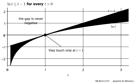
The estimate is the maximum-likelihood one. Take \({\alpha = 0}\) and drop the class index. The log likelihood of the training words of one class is \({\sum_j N_j \ln \theta_j}\), plus a constant. We show that \({\hat\theta_j = N_j/N}\) beats every other choice \(\theta\) with \({\sum_j \theta_j = 1}\). The tool is one inequality, pictured below: \({\ln t \le t - 1}\) for every \({t > 0}\). (The gap \({t - 1 - \ln t}\) has derivative \({1 - 1/t}\), negative below 1 and positive above, so its least value is 0, at \({t = 1}\).)
ML02.6.3-F3
The inequality behind maximum likelihood for word probabilities.
Compare any \(\theta\) with \(\hat\theta\), word by word, using \({t = \theta_j/\hat\theta_j}\) (words with \({N_j = 0}\) add nothing to either side and are left out):
The fourth line uses \({N_j/\hat\theta_j = N}\). The last uses \({\sum \theta_j \le 1}\) over the words kept and \({\sum N_j = N}\). So no \(\theta\) has a higher likelihood than the relative frequencies. Smoothing then adds \(\alpha\) imaginary appearances of every word, which is why \({\alpha V}\) joins the denominator.
Naive Bayes is a linear classifier. Take the log of the posterior odds for two classes. The multinomial coefficient cancels, and the log of a product of powers is a sum:
The counts enter linearly, with one weight per word, \({w_j = \ln(\theta_{1j}/\theta_{0j})}\), and a bias \({b = \ln(\pi_1/\pi_0)}\). This is the form of logistic regression on word counts. The difference is how the weights are found: naive Bayes reads them off counts in one pass, while logistic regression searches for them by gradient descent.
Worked example
Classify “free free lunch” with the corpus above, add-one smoothing and equal priors.
Word probabilities. From the counts, spam’s are \({(6, 1, 2, 5, 2, 4)/20}\) and the other class’s are \({(2, 4, 5, 2, 5, 2)/20}\), in the order free, lunch, meeting, money, team, win.
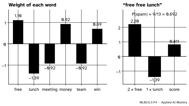
Weights. Each weight is the log of a ratio of twentieths, so the twentieths cancel:
Probability. The odds are \({e^{0.811} = 2.25 = 9/4}\), so \({p(\text{spam} \mid \vect{x}) = 9/13 = 0.692}\), matching the picture in the intuition. For “free lunch” the score is \({1.099 - 1.386 = -0.288}\), odds \({3/4}\), probability \({3/7 = 0.429}\): not spam. The second “free” flipped the decision.
Code
From scratch first: split the messages, count, smooth and take logs.
import numpy as npdocs = ["free money free win", "win free money", "free money team", "win free money meeting","team meeting lunch", "meeting team lunch free", "team lunch meeting", "win money meeting team"]y = np.array([1, 1, 1, 1, 0, 0, 0, 0]) # 1 = spamvocab =sorted({word for doc in docs for word in doc.split()})def counts(doc):return np.array([doc.split().count(word) for word in vocab])X = np.array([counts(doc) for doc in docs])alpha =1.0N = np.array([X[y == k].sum(axis=0) for k in (0, 1)]) # word counts per classtheta = (N + alpha) / (N.sum(axis=1, keepdims=True) + alpha *len(vocab))w = np.log(theta[1] / theta[0]) # one weight per wordb = np.log(np.mean(y ==1) / np.mean(y ==0))print(vocab)print("weights:", w.round(3), " bias:", b)for message in ["free free lunch", "free lunch", "win lunch meeting"]: s = b + counts(message) @ wprint(f"{message!r}: score {s:.3f}, P(spam) = {1/ (1+ np.exp(-s)):.4f}")
The library version: CountVectorizer builds the vocabulary and the count vectors, and MultinomialNB does the counting and smoothing. Its feature_log_prob_ holds \({\ln \hat\theta_{kj}}\).
The weights match the hand-built ones. “Pizza” is not in the training vocabulary, so the vectorizer drops it and “pizza free lunch” scores exactly like “free lunch”.
Naive Bayes is still a common first model for text. Training is one pass of counting, and the scikit-learn guide notes that it can be extremely fast compared with more sophisticated methods and that it has worked well in document classification and spam filtering despite its assumption. It makes a strong baseline that any more expensive model has to beat.
Explore
The module’s interactive, the two-class Gaussian explorer, sits in lesson ML02.6.4. Its duplicated feature is the continuous cousin of a word repeated in every message: evidence counted twice.
Pitfalls
ML02.6.3-F5
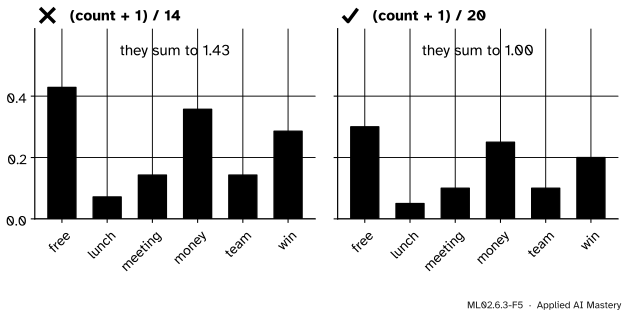
Wrong beside right. Adding one to every count without adding \(V\) to the total gives “probabilities” that sum to more than 1.
“Smoothing means adding one to each count.”
To the counts, yes, and so also to the total. Every word gets one extra appearance, so the class total grows by \(V\). Divide by 14 instead of 20 and spam’s six numbers sum to 1.43, which is not a distribution, and longer messages get inflated scores for every class.
“A word’s weight is how common it is in spam.”
The weight is the log ratio of its probabilities in the two classes. A word that is common in both, such as “the”, has a large \(\theta\) in each and a weight near 0: it says nothing about the class. “Win” is rarer than “money” in spam, but both lean towards spam because both are rarer still elsewhere.
“Fit the vectorizer on all the messages, test ones included.”
That builds the vocabulary from the test set, which leaks information and changes \(V\) and every smoothed estimate. Fit CountVectorizer on the training messages only and transform the test ones; words never seen in training are then ignored, as they should be.
Check yourself
Recall
1. What does the bag of words keep, and what does it throw away?
Show answer
It keeps how many times each vocabulary word appears and throws away their order.
2. Write the smoothed multinomial estimate of \({\theta_{kj}}\).
Show answer
\({\hat\theta_{kj} = (N_{kj} + \alpha)/(N_k + \alpha V)}\), with \(N_{kj}\) the count of word \(j\) in class \(k\), \(N_k\) the class total and \(V\) the vocabulary size.
3. Why can the multinomial coefficient \({m!/(x_1! \cdots x_V!)}\) be ignored when classifying?
Show answer
It depends only on the message, not on the class, so it is the same factor in every class’s score and cancels in Bayes’ rule.
4. What are the weight of word \(j\) and the bias of two-class multinomial naive Bayes?
Show answer
\({w_j = \ln(\theta_{1j}/\theta_{0j})}\) and \({b = \ln(\pi_1/\pi_0)}\); the log-odds are \({b + \sum_j w_j x_j}\).
5. In the corpus, why does “free free lunch” count as spam while “free lunch” does not?
Show answer
“Free” has weight \({\ln 3 = 1.099}\) and “lunch” \({\ln(1/4) = -1.386}\). One “free” loses to “lunch” (score \({-0.288}\)); two “free”s win (score \({0.811}\)).
Exercises
1.★ With the corpus and add-one smoothing, find \({p(\text{spam} \mid \text{"win lunch meeting"})}\).
The odds are 0.2, so the probability is \({0.2/1.2 = 1/6 \approx 0.167}\).
2.★★ Redo the worked example without smoothing (\({\alpha = 0}\)). Which weight breaks, and what happens to “free free lunch”?
Show solution
Spam’s probabilities become \({(5, 0, 1, 4, 1, 3)/14}\) and the other class’s \({(1, 3, 4, 1, 4, 1)/14}\). “Lunch” has \({\hat\theta = 0}\) in spam, so \({w_{\text{lunch}} = \ln(0/3) = -\infty}\). Any message containing “lunch” scores \({-\infty}\) and gets \({p(\text{spam}) = 0}\), however many times it says “free”. No other weight breaks, because every other word appears at least once in both classes.
3.★★★ Fit Bernoulli naive Bayes with add-one smoothing to the same eight messages, counting each word as present or absent. Find \({p(\text{spam})}\) for “free lunch”, and explain why “free free lunch” gets the same answer.
Show solution
Count messages, not words: with 4 messages per class, \({\hat\theta = (n_{kj} + 1)/6}\). Spam has free in 4, lunch in 0, meeting 1, money 4, team 1, win 3, so \({(5, 1, 2, 5, 2, 4)/6}\). The other class has \({(2, 4, 5, 2, 5, 2)/6}\). For “free lunch”, free and lunch are present and the other four absent:
With equal priors the posterior is \({160/288 = 5/9 \approx 0.556}\). “Free free lunch” has the same present and absent words, so the Bernoulli model gives it the same \({5/9}\): it cannot see repetition. It also lets the absent words vote, which is why it disagrees with the multinomial \({3/7}\) for “free lunch”.
Summary card
A message is a bag of rolls of each class’s word die.
ML02.6.3-F1
Repeated words count again.
Likelihood:\({p(\vect{x} \mid k) \propto \prod_j \theta_{kj}^{x_j}}\), with counts \(x_j\).
Linear: log-odds \({= b + \sum_j w_j x_j}\), with \({w_j = \ln(\theta_{1j}/\theta_{0j})}\).
Sources and next steps
Sources. Each was opened and checked against this lesson on 15 November 2026.
D. Jurafsky and J. H. Martin, Speech and Language Processing, Appendix B: Naive Bayes Classification, 3rd edition draft. Section B.1: the bag-of-words assumption, and equation B.10 with the remark that the log form makes naive Bayes a linear classifier. Section B.2: the class prior (B.11), the word estimate from counts (B.12), add-one smoothing over the whole vocabulary (B.14), and unknown test words simply ignored.
scikit-learn, Naive Bayes, User Guide section 1.9: naive Bayes has worked well in document classification and spam filtering and is fast; section 1.9.2 gives the smoothed estimate \({(N_{yi} + \alpha)/(N_y + \alpha n)}\) and calls \({\alpha = 1}\) Laplace smoothing.