Score a probability curve by how probable it makes the labels that were actually seen. Taking logarithms turns that product into a sum, the mean negative log-likelihood or cross-entropy, and shows why squared error is the wrong loss for a sigmoid.
Compute the likelihood of a set of labels under a logistic regression model.
Derive the log loss, the mean negative log-likelihood, from the likelihood step by step.
Work out the log loss of a small dataset by hand and judge its size against a coin flip.
Explain why squared error gives almost no learning signal for a confidently wrong prediction, while log loss gives a strong one.
In review. The maths and code on this page are checked by automated tests on every change, but an independent reader has not signed it off yet. Spot a mistake or a confusing step? Tell us.
The question
Lesson 1 produced a curve that turns hours of study into a probability of passing. There is one such curve for every choice of the weight and the bias. Which curve fits the six students best? The squared error that served so well for lines is the obvious way to score them, and the wrong one. What is the right one, and where does it come from?
From the last lesson
1. Write the sigmoid function. What are \(\sigma(0)\) and the range of \(\sigma\)?
Show answer
\(\sigma(z) = \frac{1}{1 + e^{-z}}\). \({\sigma(0) = \tfrac12}\), and \({0 < \sigma(z) < 1}\) for every \(z\).
2. In logistic regression, which quantity is a straight-line function of the input \(x\)?
Show answer
The log-odds: \(\ln\frac{p}{1 - p} = wx + b\).
Intuition
A model that outputs probabilities makes a kind of bet on every example. Judge it by one number per example: how much probability did it give to what actually happened?
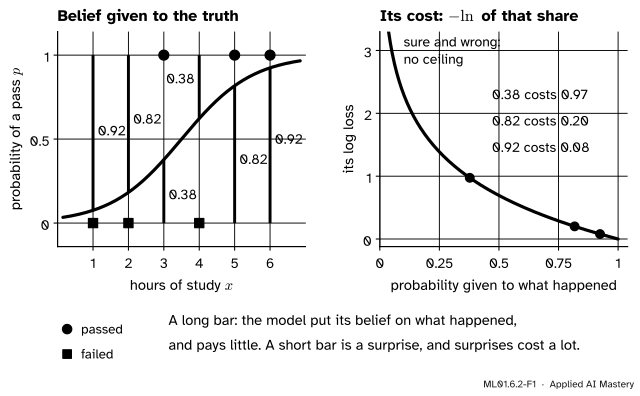
Take the model of lesson 1, \({p = {\sigma(x - 3.5)}}\). The student who studied five hours passed, and the model gave a pass probability \(0.82\): it gave \(0.82\) to the truth. The student who studied four hours failed. The model gave a pass \(0.62\), so it gave only \({1 - 0.62 = 0.38}\) to the truth.
ML01.6.2-F1
Left: the length of each bar is the probability the model gave to that student’s actual result. Right: the log loss charges each bar minus its logarithm. A full bar is free, a half bar costs \(0.69\), and the cost grows without limit as the bar shrinks to nothing.
A good curve gives a large share of its belief to the truth for every student. The log loss turns each share into a cost, minus its natural logarithm, and averages the costs. This recipe is not arbitrary. It falls out of one question: under this model, how probable were the six results we saw?
Build it up
Step 1. One student. The model says a pass has probability \(p_i\). If student \(i\) passed, the probability it gave to the truth is \(p_i\). If the student failed, it is \({1 - p_i}\). For the six students and the model \({w = 1}\), \({b = -3.5}\), the six shares are, to three places,
Step 2. All six at once. One student’s result tells us nothing about another’s once the hours are known, so the results are independent, and independent probabilities multiply. The probability of seeing exactly these six results is the product of the six shares:
This number is the likelihood of the model: the probability it gives to the whole dataset. (Results are computed before rounding. The six shares as printed multiply to \(0.0816\).)
Step 3. The best curve is the one with the highest likelihood. Different parameters give different likelihoods. Choosing the parameters that make the observed data most probable is called maximum likelihood.
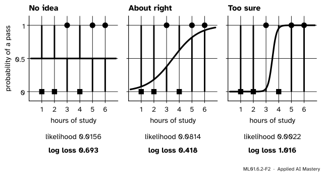
ML01.6.2-F2
Three candidate curves: \({{(w, b)} = {(0, 0)}}\), \({(1, -3.5)}\) and \({(6, -21)}\). The flat curve hedges every bet. The steep curve is certain, and twice it is certain of the wrong thing, which costs it almost everything.
Step 4. Take logarithms. A product of many numbers below \(1\) is awkward: two thousand shares of one half multiply to a number that a computer rounds to zero. The logarithm repairs this, because the logarithm of a product is the sum of the logarithms. And since \(\ln\) is increasing, the parameters with the highest likelihood also have the highest log-likelihood. Ours is \(-2.509\).
Step 5. Flip the sign and average. Every loss in this course is something to minimise, and is a mean over the examples. So change the sign of the log-likelihood and divide by \(n\): \({2.509 / 6 = 0.418}\). That is the log loss of this model.
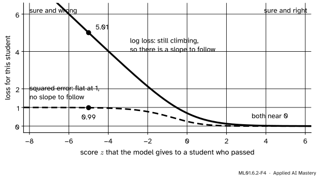
Step 6. Why not squared error? Follow one student who passed, and let the model’s score \(z\) for that student vary. The squared error is \({(1 - \sigma(z))^2}\) and the log loss is \({-\ln \sigma(z)}\).
ML01.6.2-F4
One student who passed. Where the model is sure and right, both losses are near \(0\). Where it is sure and wrong, squared error has flattened out just below \(1\), while log loss is still climbing along a straight line.
A model that is sure and wrong should get the loudest signal to change. Gradient descent listens to the slope of the loss, and on the left of the figure squared error has almost no slope.
The formal statement
NoteDefinition: the log loss
For examples \({(\cdata{x_i}, \ctruth{y_i})}\) with labels \(0\) or \(1\) and predictions \(\cmodel{p_i} = {\sigma(w x_i + b)}\),
Check both cases. If \({y_i = 1}\) it is \({p_i^{1} (1 - p_i)^{0}} = p_i\). If \({y_i = 0}\) it is \({p_i^{0} (1 - p_i)^{1}} = 1 - p_i\). These are the two shares of Step 1.
All labels. For independent examples the probabilities multiply. This is the likelihood:
Sign and mean. Multiply by \({-\tfrac{1}{n}}\). Maximising the likelihood and minimising \(L\) are now the same task.
Three facts to read off the formula.
It is never negative. Each share is at most \(1\), so its logarithm is at most \(0\), and minus that is at least \(0\). The loss is \(0\) only if every label gets probability \(1\).
A coin flip scores \({\ln 2 = 0.693}\). With \({w = 0}\) and \({b = 0}\) every \(p_i\) is \(0.5\), and \({-\ln 0.5 = \ln 2}\). On data with as many passes as fails, a loss above \(0.693\) is worse than knowing nothing.
There is no ceiling. As a share falls to \(0\), minus its logarithm grows without limit. One confident mistake can outweigh many good predictions.
Squared error against log loss. For a student who passed (\({y = 1}\)) with score \(z\), squared error is \({(1 - p)^2}\) and log loss is \({-\ln p}\):
\(z\)
\({p = \sigma(z)}\)
Squared error
Log loss
\(-10\)
\(0.0000454\)
\(0.9999\)
\(10.00\)
\(-5\)
\(0.0067\)
\(0.987\)
\(5.01\)
\(-2\)
\(0.119\)
\(0.776\)
\(2.13\)
\(0\)
\(0.5\)
\(0.25\)
\(0.69\)
\(2\)
\(0.881\)
\(0.014\)
\(0.13\)
Squared error cannot exceed \(1\) here, so it cannot tell a bad prediction from a terrible one. Moving the score from \(-10\) to \(-5\) is real progress, yet it improves only from \(0.9999\) to \(0.987\). Seen as a function of \(w\) and \(b\), it is not a bowl either: it has flat shelves on which gradient descent stalls. The log loss of logistic regression is convex, a single valley, so the methods of module ML01.5 work on it. The pitfalls section shows the difference on a real run.
Go deeper: the same loss written with the score, and the name cross-entropy
With the score. A passing student costs \({-\ln p = {\ln(1 + e^{-z})}}\) and a failing one \({\ln(1 + e^{z})}\), as exercise 3 shows. Computing the loss from \(z\) in this way never takes the logarithm of \(0\), which is one way libraries keep it finite.
The name. For two probability distributions \(q\) and \(p\) over the same outcomes, the cross-entropy is \({-\sum_k q_k \ln p_k}\). Put all of \(q\) on what happened, \({q = {(y, 1 - y)}}\), and let \(p\) be the model’s prediction, \({(p, 1 - p)}\). The sum is \({-[y \ln p + (1 - y)\ln(1 - p)]}\), the loss of one example.
Frontier note: the same loss trains language models
A language model is trained on exactly this loss, extended to many classes: minus the logarithm of the probability it gave to the token that actually came next, averaged over the text.
Worked example
The log loss of the model \({w = 1}\), \({b = -3.5}\), by hand.
The probabilities \(p_i\) come from lesson 1. For each student, pick the share that went to the truth, \(p_i\) after a pass and \({1 - p_i}\) after a fail. Its cost is minus its logarithm.
\(x_i\)
\(y_i\)
\(p_i\)
share
cost
\(1\)
\(0\)
\(0.076\)
\(0.924\)
\(0.079\)
\(2\)
\(0\)
\(0.182\)
\(0.818\)
\(0.201\)
\(3\)
\(1\)
\(0.378\)
\(0.378\)
\(0.974\)
\(4\)
\(0\)
\(0.622\)
\(0.378\)
\(0.974\)
\(5\)
\(1\)
\(0.818\)
\(0.818\)
\(0.201\)
\(6\)
\(1\)
\(0.924\)
\(0.924\)
\(0.079\)
sum
\(2.509\)
\[
L = \frac{2.509}{6} = 0.418 .
\]
(The sum uses unrounded costs. As printed they add up to \(2.508\).)
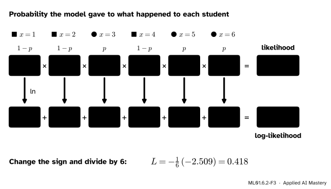
ML01.6.2-F3
The same calculation as a picture. Along the top the shares multiply to the likelihood. The logarithm takes each box down a row, where the same numbers simply add.
Two students dominate the sum: the pass after three hours and the fail after four. Each costs \(0.974\), more than the other four together. No rising curve can get both right, because the pass comes before the fail.
Is \(0.418\) good? It beats the coin flip, \(0.693\). Take the too-sure curve of Step 3, \({w = 6}\), \({b = -21}\). It is right about four students with near certainty, at almost no cost. To the truth about the other two it gives a share of only \(0.0474\), at a cost of \({-\ln 0.0474 = 3.049}\) each:
\[
L \approx \frac{3.049 + 3.049}{6} = 1.016 .
\]
That is worse than the coin flip, although, like the curve of lesson 1, it gets the same four students right.
Code
From scratch. The log loss is three lines of NumPy.
import numpy as nphours = np.array([1.0, 2.0, 3.0, 4.0, 5.0, 6.0])passed = np.array([0.0, 0.0, 1.0, 0.0, 1.0, 1.0])def sigmoid(z):return1.0/ (1.0+ np.exp(-z))def shares(w, b, x=hours, y=passed):"""The probability the model gave to what actually happened, one entry per example.""" p = sigmoid(w * x + b)return np.where(y ==1, p, 1- p)def log_loss(w, b, x=hours, y=passed):return-np.mean(np.log(shares(w, b, x, y)))print("shares:", np.round(shares(1.0, -3.5), 3))print("costs: ", np.round(-np.log(shares(1.0, -3.5)), 3))for name, (w, b) in {"no idea": (0.0, 0.0), "about right": (1.0, -3.5), "too sure": (6.0, -21.0)}.items(): q = shares(w, b)print(f"{name:12s} likelihood = {np.prod(q):.4f} log loss = {log_loss(w, b):.3f}")
shares: [0.924 0.818 0.378 0.378 0.818 0.924]
costs:  [0.079 0.201 0.974 0.974 0.201 0.079]
no idea      likelihood = 0.0156   log loss = 0.693
about right  likelihood = 0.0814   log loss = 0.418
too sure     likelihood = 0.0022   log loss = 1.016
Next, why a computer needs the logarithm, and the table that compares the two losses.
print("0.5 ** 1000 =", 0.5**1000)print("0.5 ** 2000 =", 0.5**2000, " but the sum of 2000 logs is", round(2000* np.log(0.5), 1))print("\n z p squared log loss")for z in [-10.0, -5.0, -2.0, 0.0, 2.0]: p = sigmoid(z)print(f"{z:5.0f}{p:7.5f}{(1- p) **2:7.4f}{-np.log(p):8.2f}")
0.5 ** 1000 = 9.332636185032189e-302
0.5 ** 2000 = 0.0   but the sum of 2000 logs is -1386.3

    z        p   squared   log loss
  -10  0.00005    0.9999      10.00
   -5  0.00669    0.9867       5.01
   -2  0.11920    0.7758       2.13
    0  0.50000    0.2500       0.69
    2  0.88080    0.0142       0.13
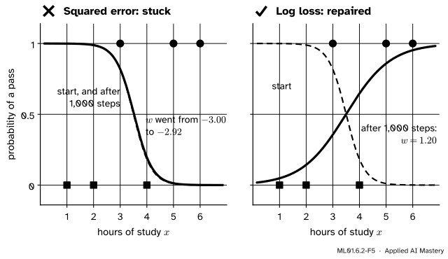
Now the experiment behind Step 6. Start both losses from the same confidently wrong curve, \({w = -3}\), \({b = 10.5}\), sure that little study means a pass, and run gradient descent on each. The slopes are measured with the finite-difference recipe of ML01.5.2, so no formula for them is needed yet.
def squared_error(w, b):return np.mean((sigmoid(w * hours + b) - passed) **2)def descend(loss, w, b, lr=0.3, steps=1000, h=1e-5):for _ inrange(steps): dw = (loss(w + h, b) - loss(w - h, b)) / (2* h) # measured slope along w db = (loss(w, b + h) - loss(w, b - h)) / (2* h) # measured slope along b w, b = w - lr * dw, b - lr * dbreturn w, bfor name, loss in [("squared error", squared_error), ("log loss", log_loss)]: w, b = descend(loss, -3.0, 10.5)print(f"{name:13s}: loss {loss(-3.0, 10.5):.4f} -> {loss(w, b):.4f}, w = {w:6.3f}, b = {b:6.3f}")
squared error: loss 0.6701 -> 0.6699,  w = -2.916, b = 10.256
log loss     : loss 4.0710 -> 0.4130,  w =  1.197, b = -4.184
After a thousand steps squared error has moved \(w\) from \(-3\) to \(-2.92\): the curve is still upside down. Log loss has turned it the right way up.
Last, the library version. scikit-learn’s log_loss takes the labels and the predicted probabilities, and returns the mean by default. Computed from the score, as in the “go deeper” note, the loss stays finite where the plain formula does not.
from sklearn.metrics import log_loss as sk_log_lossp = sigmoid(1.0* hours -3.5)print("scikit-learn:", round(sk_log_loss(passed, p), 6), " from scratch:", round(log_loss(1.0, -3.5), 6))z = np.array([40.0]) # a student who failed, scored +40with np.errstate(divide="ignore"):print("plain formula: ", -np.log(1- sigmoid(z))) # sigmoid(40) rounds to exactly 1print("from the score:", np.logaddexp(0.0, z)) # ln(1 + e^z), computed safely
scikit-learn: 0.418127   from scratch: 0.418127
plain formula:  [inf]
from the score: [40.]
Explore
The sigmoid and boundary explorer is in lesson 3. Its bar chart shows the log loss of every student and their mean. It opens at \({w = 1}\), \({b = -3.5}\): read off \(0.418\). Then set \({w = 6}\) and \({b = -21}\), the too-sure curve. Two bars tower over the rest and push the mean to \(1.016\), above the coin-flip line at \(0.693\).
Pitfalls
ML01.6.2-F5
Wrong beside right. The same model, the same upside-down start, the same learning rate and the same thousand steps. Only the loss differs.
“Squared error worked for lines, so it will work for the sigmoid.”
On a confidently wrong prediction the squared error of a sigmoid is nearly flat, so gradient descent gets almost no signal exactly where it needs the most. In the figure it is stuck on a shelf: after a thousand steps its loss has gone from \(0.6701\) to \(0.6699\). Log loss is steep there, and falls from \(4.07\) to \(0.413\) in the same number of steps.
“Two models that make the same mistakes are equally good.”
The gentle curve and the too-sure curve get the same four students right, yet their log losses are \(0.418\) and \(1.016\). A model that says \(0.95\) and is wrong is worse than one that says \(0.62\) and is wrong, because someone will act on the \(0.95\). Module ML01.7 measures answers. The log loss measures the honesty of the probabilities.
“A log loss of 0.69 always means a coin flip.”
Only when the two classes are equally common. If one student in ten passes, always predicting \(0.1\) scores \(0.325\), so a model must beat that. Exercise 2 works it out.
Check yourself
Recall
1. What is the likelihood of a model on a dataset?
Show answer
The probability the model gives to the labels that were actually observed: the product, over the examples, of \(p_i\) for each label \(1\) and \({1 - p_i}\) for each label \(0\).
3. Give two reasons for taking the logarithm of the likelihood.
Show answer
It turns a product into a sum, which is easier to differentiate, and it stops a product of many small numbers rounding to zero. It does not change which parameters are best, because the logarithm is increasing.
4. What is the log loss of a model that predicts \(0.5\) for every example?
5. For a prediction that is confident and wrong, how do squared error and log loss differ?
Show answer
Squared error flattens out just below \(1\), so it has almost no slope and gives almost no signal. Log loss keeps growing, roughly in a straight line in the score, so its slope stays large.
Exercises
1.★ Three examples have labels \({y = {(1, 0, 1)}}\) and a model predicts \({p = {(0.9, 0.2, 0.6)}}\). Compute the likelihood and the log loss.
Show solution
The shares given to the truth are \(0.9\), \({1 - 0.2 = 0.8}\) and \(0.6\). The likelihood is \({0.9 \times 0.8 \times 0.6} = 0.432\). The costs are \({-\ln 0.9 = 0.105}\), \({-\ln 0.8 = 0.223}\) and \({-\ln 0.6 = 0.511}\), so \(L = {(0.105 + 0.223 + 0.511)/3} = 0.280\). Check: \({-\ln(0.432)/3 = 0.280}\).
2.★★ A model ignores the input and predicts the same probability \(p\) for everyone. Among \(n\) examples, \(k\) have label \(1\). Find the \(p\) with the lowest log loss. Then give the loss of that model when one example in ten has label \(1\).
Show solution
The \(k\) examples with label \(1\) each cost \({-\ln p}\), and the other \({n - k}\) each cost \({-\ln(1 - p)}\):
\[
\begin{aligned}
L(p) &= -\frac{1}{n}\Big[\, k \ln p \\
&\qquad + (n - k)\ln(1 - p) \,\Big] .
\end{aligned}
\]
Set the derivative to zero: \(\frac{dL}{dp} = {-\frac{1}{n}\Big[\frac{k}{p} - \frac{n - k}{1 - p}\Big]} = 0\), so \({{k(1 - p)} = {(n - k)p}}\), which gives \({k = np}\) and \({p = k/n}\). The best constant prediction is the share of ones in the data. (The second derivative is positive, so this is a minimum.)
3.★★★ Show that the loss of one example can be written with the score alone as \(\ell = {\ln(1 + e^{z}) - y z}\), for both \({y = 1}\) and \({y = 0}\). Use it to explain the straight line on the left of the figure in Step 6.
Show solution
Case \({y = 0}\). The loss is \({-\ln(1 - p)}\). From lesson 1, \(1 - p = {\sigma(-z)} = \frac{1}{1 + e^{z}}\), so \({-\ln(1 - p)} = {\ln(1 + e^{z})}\), which is the formula with \({y = 0}\).
Case \({y = 1}\). The loss is \({-\ln p = {\ln(1 + e^{-z})}}\). Write \(1 + e^{-z} = \frac{e^{z} + 1}{e^{z}}\). Then
For a passing student and a very negative score, \(e^{z}\) is nearly \(0\), so \({{\ln(1 + e^{z})} \approx 0}\) and \({\ell \approx -z}\): a straight line of slope \(-1\). At \({z = -5}\) the exact value is \(5.007\).
Summary card
Score a model by the probability it gave to what happened.
ML01.6.2-F1
Belief given to the truth, and its cost.
Likelihood.\({\prod_i p_i^{\,y_i}(1 - p_i)^{\,1 - y_i}}\): the probability of the observed labels.
Benchmarks.\(0\) is perfect, \({\ln 2 = 0.693}\) is a coin flip, and there is no upper limit.
By hand. For \({w = 1}\), \({b = -3.5}\): likelihood \(0.0814\), log-likelihood \(-2.509\), \({L = 0.418}\).
Why not squared error. It is flat for confident mistakes, so it gives no slope to follow.
Sources and next steps
Sources. Each was opened and checked against this lesson on 12 November 2026.
Daniel Jurafsky and James H. Martin, Speech and Language Processing, 3rd edition draft of 19 August 2026, Chapter 4, Section 4.5. Derives the cross-entropy loss in the steps used here: the probability of one label, \({\hat{y}^{y}(1 - \hat{y})^{1 - y}}\) (equation 4.17), its logarithm (4.18) and the change of sign (4.19). Sections 4.7 and 4.8 extend the loss to many classes, such as the next word, as minus the log probability of the correct class (4.39).
Tengyu Ma and Andrew Ng, CS229 Lecture Notes, Stanford University, Section 2.1. Writes the likelihood as a product over independent training examples and takes its logarithm (equation 2.1).
Roger Grosse, Lecture 4: Training a Classifier, CSC321, University of Toronto, 2018. Section 2.3 makes the argument of Step 6 with a positive example scored \({z = -5}\): “the more confident the wrong prediction, the smaller the gradient”. Section 2.5 computes the loss from the score (equation 17). Section 4 says the logistic regression objective is convex, and the logistic function with least squares is not.
scikit-learn 1.9 documentation, sklearn.metrics.log_loss. Uses the natural logarithm, returns the mean loss per sample by default, and clips the probabilities away from 0 and 1.