A full model of which of 500 words an email contains needs more numbers than there are atoms in the universe. Assume the words are independent within each class and it needs one number per word. Build Bernoulli naive Bayes on the inbox, in logs, with add-one smoothing.
ML02.6.2L2 Intermediate25 minIn review (what this means)
The maths and code on this page are checked by automated tests on every change, but an independent reader has not signed it off yet. Spot a mistake or a confusing step? Tell us.
State the naive Bayes assumption and count the parameters it saves: d per class instead of 2^d - 1 for d binary features.
Classify an email with Bernoulli naive Bayes, including the factors for the words it does not contain.
Compute naive Bayes scores as sums of logs, and explain why the plain product fails for long inputs.
Explain how a zero count wipes out a class and how additive smoothing with pseudo-counts prevents it.
The question
A spam filter describes each email by which of its 500 vocabulary words appear in it. The Bayes classifier of the last lesson needs \({p(\vect{x} \mid \text{spam})}\) for every possible pattern of 500 yes-or-no answers. There are \({2^{500}}\) such patterns, far more than the emails ever written. How can a filter work at all?
From the last lesson
1. What does the Bayes classifier predict, and why is it the best possible?
Show answer
The class with the largest \({\pi_k\, p(\vect{x} \mid k)}\). At every \(x\) it leaves only the smaller weighted density as error, so no classifier has a lower expected error rate.
2. In the worked example, the two likelihoods were equal at \({x = 3}\). What was the posterior there?
Show answer
The prior, 0.4. When the evidence is the same under both classes, it does not move the probability.
Intuition
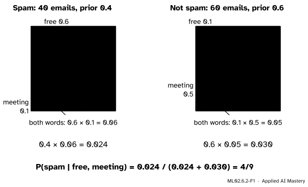
The way out is a bold simplification. Assume that, once you know the class, the words appear independently of each other. Then the chance that a spam email contains both “free” and “meeting” is just the chance of “free” in spam times the chance of “meeting” in spam.
ML02.6.2-F1
The naive assumption on the inbox of M06.3 and M06.4. Inside each class, “free” splits the square one way and “meeting” the other, so every cell is a product. The yellow cells, weighted by the priors, give the posterior 4/9.
This is the naive Bayes assumption. It is called naive because it is rarely true: an email with “free” is more likely to also say “offer”. But it turns an impossible estimation problem into \({d}\) easy ones per class, one for each word, and the resulting classifier often works well.
Build it up
Step 1. Features as yes-or-no answers. Write the email as a vector \({\vect{x} = (x_1, \dots, x_d)}\) with \({x_j = 1}\) if word \(j\) appears and \({x_j = 0}\) if not. In the inbox, \({d = 2}\): \(x_1\) is “free” and \(x_2\) is “meeting”.
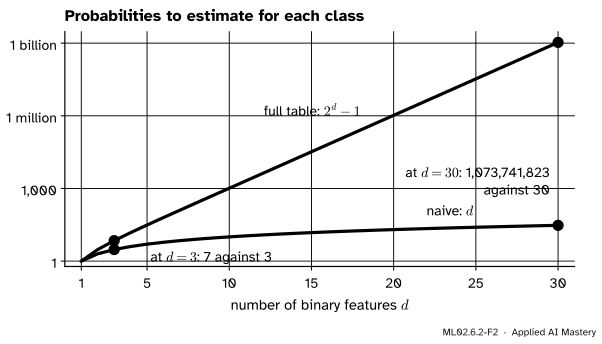
Step 2. The full table is too big. Without an assumption, \({p(\vect{x} \mid k)}\) is a table with one probability for each of the \({2^d}\) patterns. They must sum to 1, so \({2^d - 1}\) of them are free to choose. That is 3 for two words, but over a billion for thirty.
ML02.6.2-F2
Numbers to estimate for each class. The full table doubles with every new feature; the naive model adds one. Every one of those numbers has to be learned from labelled examples.
Step 3. Conditional independence. Two events are conditionally independent given \(C\) when \({\Prob(A \cap B \mid C) = \Prob(A \mid C)\,\Prob(B \mid C)}\) (M06.3.4). Assume this for all the words given the class. The likelihood of the whole email becomes a product of one factor per word:
Step 4. One coin per word. Each factor is a Bernoulli variable (M06.8.1) with its own probability \({\theta_{kj} = \Prob(x_j = 1 \mid k)}\). A present word contributes \(\theta_{kj}\) and an absent word contributes \({1 - \theta_{kj}}\). One formula covers both:
Absent words count. Not containing “meeting” is evidence too: 90% of spam lacks it, but only half of the other emails do.
The formal statement
NoteDefinition: Bernoulli naive Bayes
For binary features \(x_j\) and classes \({k = 1, \dots, K}\), with priors \(\pi_k\) and word probabilities \(\theta_{kj}\), the Bernoulli naive Bayes classifier predicts the class with the largest score
The parameters are estimated by counting. If \(n_k\) training examples are in class \(k\) and \(n_{kj}\) of them have feature \(j\), then with smoothing constant \({\alpha \ge 0}\),
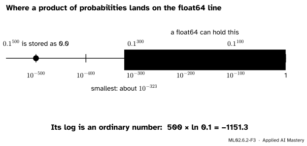
Why logs. The score is the log of \({\pi_k\, p(\vect{x} \mid k)}\): the log of a product is the sum of the logs. The log changes nothing about which class is largest, because it only ever increases. It does change whether a computer can hold the number. A float64 cannot store a positive number below about \({10^{-323}}\), and a product of 500 probabilities near 0.1 is about \({10^{-500}}\). It is stored as exactly 0.0, for every class, and the posterior becomes \({0/0}\).
ML02.6.2-F3
A product of many probabilities underflows. The sum of their logs is a modest negative number that a float holds with ease.
To turn scores back into probabilities, subtract the largest score before exponentiating. This log-sum-exp trick divides top and bottom by the same factor \({e^{s_{\max}}}\), so nothing changes but the size of the numbers:
The largest term in the denominator is now \({e^0 = 1}\), so it cannot underflow.
Why smoothing. With \({\alpha = 0}\) the estimate is the raw share \({n_{kj}/n_k}\), the maximum likelihood estimate of a Bernoulli probability (S02.3.2). If a word never appears in the training spam, its \({\hat\theta}\) is 0, its log is \({-\infty}\), and every future email containing it scores spam as impossible, whatever else it says. Adding \(\alpha\) to the count with the word and \(\alpha\) to the count without it acts like \({2\alpha}\) imaginary extra emails per class, half with the word and half without. These are pseudo-counts. With \({\alpha = 1}\) it is Laplace smoothing, or add-one.
Go deeper: smoothing as a Bayesian estimate
Put a Beta\({(\alpha, \alpha)}\) prior on \(\theta\), a density proportional to \({\theta^{\alpha - 1}(1 - \theta)^{\alpha - 1}}\), symmetric about one half. After \(n_{kj}\) emails with the word out of \(n_k\), the likelihood is \({\theta^{n_{kj}}(1 - \theta)^{n_k - n_{kj}}}\), and the posterior is proportional to the product, \({\theta^{n_{kj} + \alpha - 1}(1 - \theta)^{n_k - n_{kj} + \alpha - 1}}\). That is a Beta\({(n_{kj} + \alpha,\; n_k - n_{kj} + \alpha)}\) density, whose mean is \({(n_{kj} + \alpha)/(n_k + 2\alpha)}\): exactly the smoothed estimate. So add-one smoothing is the posterior mean under a flat prior on \(\theta\), and \(\alpha\) says how strongly you believe, before seeing data, that each word is as likely present as absent.
Worked example
The inbox has 100 emails, 40 spam. “Free” is in 24 spam and 6 others; “meeting” is in 4 spam and 30 others. An email contains both words. Is it spam?
Estimates, with \({\alpha = 0}\). The priors are 0.4 and 0.6. For spam, \({\hat\theta_{\text{free}} = 24/40 = 0.6}\) and \({\hat\theta_{\text{meeting}} = 4/40 = 0.1}\). For the others, \({6/60 = 0.1}\) and \({30/60 = 0.5}\).
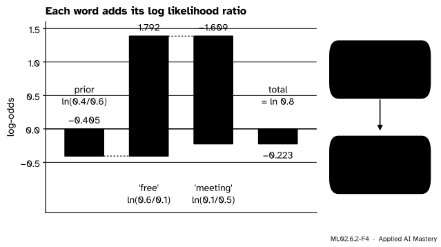
Log-odds, one term at a time. For two classes it is simplest to subtract the two scores. Both words are present, so only the \(\theta\) factors appear, and each word adds the log of a ratio:
the answer of the Bayes table in M06.4.4. The email is classed as not spam.
With add-one smoothing. Now \({\hat\theta_{\text{free}} = 25/42}\) and \({\hat\theta_{\text{meeting}} = 5/42}\) for spam, and \({7/62}\) and \({31/62}\) for the others. The products are \({0.4 \times \tfrac{25}{42} \times \tfrac{5}{42} = 0.02834}\) and \({0.6 \times \tfrac{7}{62} \times \tfrac{31}{62} = 0.03387}\), so the posterior is \({0.02834/0.06221 = 0.456}\). Smoothing nudged every estimate a little towards one half and the answer moved from 0.444 to 0.456. With 40 and 60 emails per class, one imaginary email barely matters.
Code
A from-scratch Bernoulli naive Bayes that works in logs throughout, trained on the 100 emails built as in M06.4.4.
import numpy as npspam = np.zeros((40, 2), dtype=int)spam[:24, 0] =1# 24 spam emails say 'free'spam[20:24, 1] =1# 4 spam emails say 'meeting'ham = np.zeros((60, 2), dtype=int)ham[:6, 0] =1# 6 others say 'free'ham[30:, 1] =1# 30 others say 'meeting'X = np.vstack([ham, spam])y = np.array([0] *60+ [1] *40) # 1 = spamdef fit(X, y, alpha): classes = np.unique(y) prior = np.array([np.mean(y == k) for k in classes]) theta = np.array([(X[y == k].sum(axis=0) + alpha) / ((y == k).sum() +2* alpha) for k in classes])return prior, thetadef scores(X, prior, theta):"""s_k = ln pi_k + sum_j [x_j ln theta_kj + (1 - x_j) ln(1 - theta_kj)], one column per class."""with np.errstate(divide="ignore"): # ln 0 = -inf is allowed when alpha = 0return np.log(prior) + X @ np.log(theta).T + (1- X) @ np.log(1- theta).Tdef posterior(s):"""Log-sum-exp: subtract the largest score before exponentiating.""" e = np.exp(s - s.max(axis=1, keepdims=True))return e / e.sum(axis=1, keepdims=True)email = np.array([[1, 1]]) # contains both wordsfor alpha in (0, 1): prior, theta = fit(X, y, alpha)print(f"alpha = {alpha}: P(spam | free, meeting) = {posterior(scores(email, prior, theta))[0, 1]:.4f}")
scikit-learn’s BernoulliNB uses the same formulas. Its smoothing constant is alpha, and it estimates the priors from the class shares without smoothing them.
from sklearn.naive_bayes import BernoulliNBmodel = BernoulliNB(alpha=1.0).fit(X, y)print("BernoulliNB:", model.predict_proba(email)[0, 1].round(4))print("theta for spam:", np.exp(model.feature_log_prob_[1]).round(4))
BernoulliNB: 0.4556
theta for spam: [0.5952 0.119 ]
Now the reason for logs. Give a long email 500 words, each with a probability between 0.01 and 0.2 under each class, and compare the plain product with the sum of logs.
products: [0. 0.]
posterior from products: [nan nan]
log scores: [-1192.7 -1218.2]
posterior from logs: [[1. 0.]]
The products are exactly zero, so the posterior is nan. The log scores, below \({-900}\), are ordinary numbers, and the posterior they give is well defined.
Explore
The module’s interactive, the two-class Gaussian explorer, sits in lesson ML02.6.4. Its “duplicate the feature” button shows what the naive assumption costs when two features carry the same evidence, the danger hiding in the product of this lesson.
Pitfalls
ML02.6.2-F5
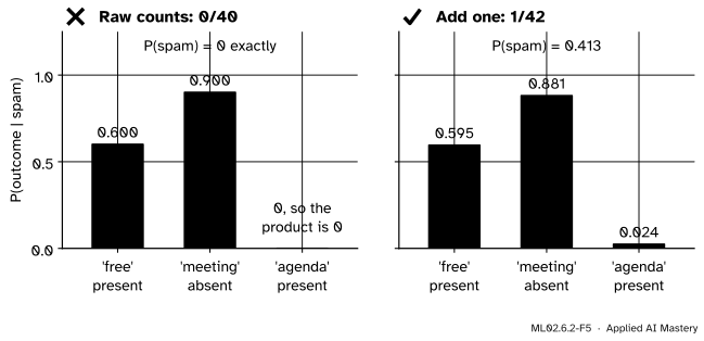
Wrong beside right. “Agenda” never appeared in the 40 training spam emails. Raw counts make one factor zero and the posterior of spam exactly 0. Add-one smoothing keeps the other evidence alive.
“A word never seen in spam proves an email is not spam.”
Suppose “agenda” is in none of the 40 spam emails and in 12 of the 60 others. With raw counts, \({\hat\theta = 0}\) for spam, and an email with “free” and “agenda” gets \({p(\text{spam}) = 0}\), however spammy the rest of it is. One spammer who writes “agenda” walks straight through. With \({\alpha = 1}\) the same email gets 0.413. A zero count says “not seen in 40 tries”, not “impossible”.
“Only the words in the email matter.”
In the Bernoulli model every vocabulary word votes, present or absent. An email with “free” but without “meeting” gets \({p(\text{spam}) = 36/41 = 0.878}\), higher than the 0.8 that “free” alone gives in M06.3, because lacking “meeting” is typical of spam. The multinomial model of the next lesson, by contrast, ignores absent words.
“Multiply the probabilities, then normalise.”
Fine for two words, broken for five hundred: the products underflow to 0 and the result is nan. Always add logs, and subtract the largest score before exponentiating.
Check yourself
Recall
1. State the naive Bayes assumption.
Show answer
The features are conditionally independent given the class, so \({p(\vect{x} \mid k) = \prod_j p(x_j \mid k)}\).
2. How many probabilities per class does a full model of \(d\) binary features need, and how many does Bernoulli naive Bayes need?
Show answer
\({2^d - 1}\) for the full table, and \(d\) for naive Bayes, one \(\theta_{kj}\) per feature.
3. What factor does an absent word contribute in Bernoulli naive Bayes?
Show answer
\({1 - \theta_{kj}}\), the probability that a class-\(k\) example lacks word \(j\).
4. Why does code add logs instead of multiplying probabilities?
Show answer
A product of many small probabilities underflows to 0.0 in floating point. The sum of their logs is an ordinary number, and the log keeps the order of the scores.
5. What is the add-one estimate of \({\theta_{kj}}\), and what problem does it fix?
Show answer
\({(n_{kj} + 1)/(n_k + 2)}\). It stops a word that never appeared in a class from giving that class probability zero.
Exercises
1.★ With raw counts, find \({p(\text{spam} \mid \text{no free, meeting})}\) for the inbox.
Show solution
“Free” is absent, so its factors are \({1 - 0.6 = 0.4}\) for spam and \({1 - 0.1 = 0.9}\) for the others. The products are \({0.4 \times 0.4 \times 0.1 = 0.016}\) and \({0.6 \times 0.9 \times 0.5 = 0.27}\), so the posterior is \({0.016/0.286 = 8/143 \approx 0.056}\).
2.★★ A filter uses 500 words and two classes. How many numbers does Bernoulli naive Bayes learn in all? How many would a full table of word patterns need?
Show solution
Naive Bayes: 500 values of \(\theta\) for each class, 1,000 in all, plus one prior (the second is one minus the first), so 1,001. The full table: \({2^{500} - 1}\) free probabilities per class, so \({2(2^{500} - 1) + 1}\), about \({6.5 \times 10^{150}}\) numbers.
3.★★★ In the 100 emails as the code builds them, count the emails that contain both words, by class. What would a full table of the two words give for \({p(\text{spam} \mid \text{free, meeting})}\)? What does this say about the naive assumption here?
Show solution
Rows 20 to 23 of the spam array have both words: 4 of 40, so \({p(\text{both} \mid \text{spam}) = 0.1}\), not the naive \({0.6 \times 0.1 = 0.06}\). No row of ham has both: “free” is in rows 0 to 5 and “meeting” in rows 30 to 59. So \({p(\text{both} \mid \text{not}) = 0}\), not \({0.1 \times 0.5 = 0.05}\). The full table gives
The words are far from independent within each class here, and the full table, built on just four emails, says “certainly spam”. Naive Bayes says 4/9. Neither is trustworthy on so few emails, which is the point: the full table has too little data per cell, and the naive model ignores the pattern.
Summary card
Within a class, multiply one probability per word.
Sources. Each was opened and checked against this lesson on 15 November 2026.
G. James, D. Witten, T. Hastie and R. Tibshirani, An Introduction to Statistical Learning, 2nd edition. Section 4.4.4 states the naive Bayes assumption, the product form (4.29) and the posterior (4.30), estimates a qualitative predictor by class proportions, and explains the gain as less variance for some bias.
D. Jurafsky and J. H. Martin, Speech and Language Processing, Appendix B: Naive Bayes Classification, 3rd edition draft. Equation B.7 is the naive Bayes assumption; B.10 moves to log space “to avoid underflow”; B.13 shows a zero count making a class impossible “no matter the other evidence”; B.14 is add-one smoothing.
scikit-learn, Naive Bayes, User Guide section 1.9.4: the Bernoulli rule, which “explicitly penalizes the non-occurrence” of a feature, and the BernoulliNB reference for alpha (Laplace or Lidstone smoothing).