The widest street becomes an optimisation problem: minimise half the squared length of w while every point stays off the street. Lagrange multipliers turn it into a dual problem whose solution gives each point a weight, zero for all but the support vectors.
ML02.7.2L2 Intermediate25 minIn review (what this means)
The maths and code on this page are checked by automated tests on every change, but an independent reader has not signed it off yet. Spot a mistake or a confusing step? Tell us.
State the hard-margin primal problem and explain why minimising half the squared norm of w gives the widest street.
Form the Lagrangian, set its derivatives to zero to get w as a weighted sum of the data and the condition that the weights balance, and derive the dual problem.
Use complementary slackness to explain why only support vectors get a non-zero weight, and recover b from a support vector.
Solve the dual of a small problem by hand and with scipy.optimize.minimize, and match the result against scikit-learn’s SVC.
The question
The angle scan of the last lesson found the widest street for six points in the plane. A medical dataset has 30 features, and no one can scan the angles of a 30-dimensional space. How do we turn “find the widest street” into a problem a solver can handle in any dimension, and why does its answer name the support vectors for us?
From the last lesson
1. How wide is the street of the classifier \({\vect{w} \cdot \vect{x} + b}\) once the closest points score \(\pm 1\)?
Show answer
\({2 / \norm{\vect{w}}}\). Each edge lies \({1 / \norm{\vect{w}}}\) from the centre line.
2. Which of the six points are support vectors?
Show answer
\({(1, 0)}\), \({(0, 1)}\) and \({(2, 2)}\), the three points on the edges of the street.
Intuition
A wide street means a short weight vector, so we look for the shortest \(\vect{w}\) that keeps every point off the street. Every point brings one rule: stay on your own side, at a score of at least \(1\). Most rules are met with room to spare. A few, those of the points on the edges, are met exactly, and those are the rules that hold the answer in place.
Lagrange’s method gives each rule a weight \(\alpha_i\), which measures how hard that rule pushes on the answer. A rule with room to spare does not push at all, so its weight is zero.
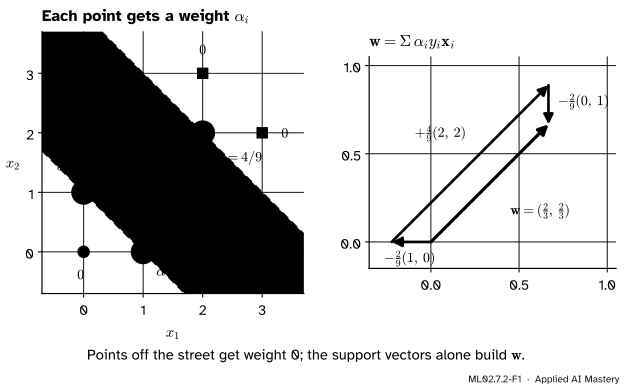
ML02.7.2-F1
The answer of this lesson. Each point gets a weight \(\alpha_i\): zero off the street, positive on its edges. The weight vector is the weighted sum of the support vectors, with sign \(y_i\).
The picture shows the punchline before the algebra: \(\vect{w}\) is built from the support vectors alone. Delete \({(0, 0)}\), \({(3, 2)}\) and \({(2, 3)}\) from the training set and nothing changes. A trained SVM only needs to keep its support vectors.
Build it up
Step 1. The primal problem. By lesson 1 the street is \({2 / \norm{\vect{w}}}\) wide when every point satisfies \({y_i (\vect{w} \cdot \vect{x}_i + b) \ge 1}\). Making \({2 / \norm{\vect{w}}}\) as large as possible is the same as making \(\norm{\vect{w}}\) as small as possible, and also the same as making \({\tfrac{1}{2}\norm{\vect{w}}^2}\) as small as possible. The square removes the root, and the \(\tfrac{1}{2}\) cancels the \(2\) that differentiating brings down. This is a quadratic programme: a quadratic objective with linear constraints.
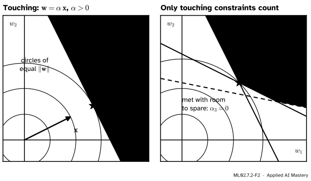
Step 2. One constraint, pictured. Drop the bias for a moment, so that \(\vect{w}\) lives in a plane we can draw. Minimise \({\tfrac{1}{2}\norm{\vect{w}}^2}\) subject to one rule \({\vect{w} \cdot \vect{x} \ge 1}\). The contours of the objective are circles around the origin. Grow a circle until it first touches the allowed half-plane: the touching point is the answer.
ML02.7.2-F2
Lagrange multipliers for inequality rules. Left: at the answer, the gradient of the objective points along the normal of the touching rule. Right: with several rules, it is a non-negative combination of the normals of the rules that touch; a rule that does not touch gets weight \(0\).
At the touching point the circle and the line are tangent, so their normals are parallel. The normal of the circle is the gradient of \({\tfrac{1}{2}\norm{\vect{w}}^2}\), which is \(\vect{w}\) itself. The normal of the line is \(\vect{x}\). So \({\vect{w} = \alpha\,\vect{x}}\) for some number \(\alpha\), and \({\alpha > 0}\) because the circle grows outwards into the allowed side.
Step 3. Several constraints. With several rules the answer may sit at a corner where two touch. Then \(\vect{w}\) is a combination \({\alpha_1 \vect{x}_1 + \alpha_2 \vect{x}_2}\) with both weights non-negative. A rule that does not touch could be deleted without moving the answer, so its weight is \(0\). M08.7 and M08.8 prove this in general; here we use it.
The formal statement
Primal. For examples \((\vect{x}_i, y_i)\) with \({y_i \in \{-1, +1\}}\), \({i = 1, \dots, n}\):
\[
\begin{aligned}
&\min_{\vect{w},\,b}\ \ \tfrac{1}{2}\norm{\cparam{\vect{w}}}^2 \quad \text{subject to} \\
&y_i\,(\cparam{\vect{w}} \cdot \vect{x}_i + \cparam{b}) \ge 1
\ \text{ for all } i .
\end{aligned}
\]
The Lagrangian. Give rule \(i\) a multiplier \({\alpha_i \ge 0}\) and subtract each rule’s surplus. The result is a function \({L(\vect{w}, b, \vect{\alpha})}\):
\[
\begin{aligned}
L &= \tfrac{1}{2}\norm{\vect{w}}^2 \\
&\quad - \sum_i \cparam{\alpha_i}\,\big[y_i(\vect{w} \cdot \vect{x}_i + b) - 1\big] .
\end{aligned}
\]
Stationarity. Set the derivatives with respect to \(\vect{w}\) and \(b\) to zero. The gradient of \({\tfrac{1}{2}\norm{\vect{w}}^2}\) is \(\vect{w}\) and the gradient of \({\vect{w} \cdot \vect{x}_i}\) is \(\vect{x}_i\), so
Now substitute the two conditions. The third piece is \(0\). For the first two, write \({\vect{w} = \sum_j \alpha_j y_j \vect{x}_j}\) and name the double sum
Then \({\tfrac{1}{2}\,\vect{w} \cdot \vect{w} = \tfrac{1}{2}S}\), and \({\sum_i \alpha_i y_i\, \vect{w} \cdot \vect{x}_i = S}\) as well, because each is the same double sum. So the first two pieces leave \({\tfrac{1}{2}S - S = -\tfrac{1}{2}S}\), and the dual problem is
Why the dual gives the right answer. Take any \((\vect{w}, b)\) that meets every rule and any \({\vect{\alpha} \ge 0}\) with \({\sum_i \alpha_i y_i = 0}\). Each bracket in \(L\) is at least \(0\), so \({L \le \tfrac{1}{2}\norm{\vect{w}}^2}\), and the dual objective is the smallest \(L\) over all \((\vect{w}, b)\), which is smaller still. So every dual value is at most every primal value. For this problem, a convex quadratic with linear rules and at least one feasible point, the two optimal values are equal (M08.8), and the worked example checks it.
Complementary slackness. At the optimum, each product is zero:
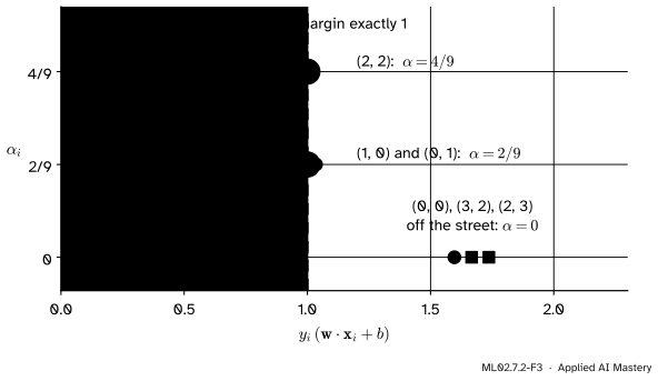
If point \(i\) is off the street, the bracket is positive, so \({\alpha_i = 0}\). If \({\alpha_i > 0}\), the bracket is zero and the point is on an edge. The points with \({\alpha_i > 0}\) are the support vectors.
ML02.7.2-F3
Complementary slackness on the six points. Every point is either on an edge of the street, with \({y_i f(\vect{x}_i) = 1}\), or has \({\alpha_i = 0}\).
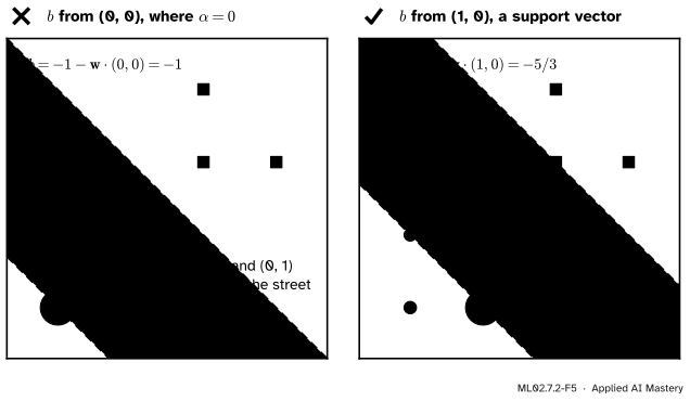
Recovering \(b\). For a support vector \(\vect{x}_s\), \({y_s(\vect{w} \cdot \vect{x}_s + b) = 1}\). Multiply both sides by \(y_s\) and use \({y_s^2 = 1}\): \({b = y_s - \vect{w} \cdot \vect{x}_s}\).
Predicting. Substituting \(\vect{w}\) into the score gives
The data enter both the dual and the prediction only through dot products \({\vect{x}_i \cdot \vect{x}_j}\). This is the door that module ML02.8 opens: replace each dot product by a kernel and the same algorithm draws curved boundaries.
Go deeper: a useful identity: the length of w
Take the dot product of \({\vect{w} = \sum_i \alpha_i y_i \vect{x}_i}\) with \(\vect{w}\):
The second line uses \({\vect{w} \cdot \vect{x}_i = y_i - b}\), which holds for every point with \({\alpha_i > 0}\) (the others contribute \(0\) anyway). The last step uses \({y_i^2 = 1}\) and \({\sum_i \alpha_i y_i = 0}\). So the width is \({2 / \sqrt{\sum_i \alpha_i}}\), and the optimal dual value is \({\sum_i \alpha_i - \tfrac{1}{2}\sum_i \alpha_i = \tfrac{1}{2}\norm{\vect{w}}^2}\), equal to the primal value.
Worked example
The six points. Number them \({\vect{x}_1 = (0, 0)}\), \({\vect{x}_2 = (1, 0)}\), \({\vect{x}_3 = (0, 1)}\) with \({y = -1}\), and \({\vect{x}_4 = (2, 2)}\), \({\vect{x}_5 = (3, 2)}\), \({\vect{x}_6 = (2, 3)}\) with \({y = +1}\). Lesson 1 suggests that \(\vect{x}_2\), \(\vect{x}_3\) and \(\vect{x}_4\) are the support vectors, so guess \({\alpha_1 = \alpha_5 = \alpha_6 = 0}\) and check the guess at the end.
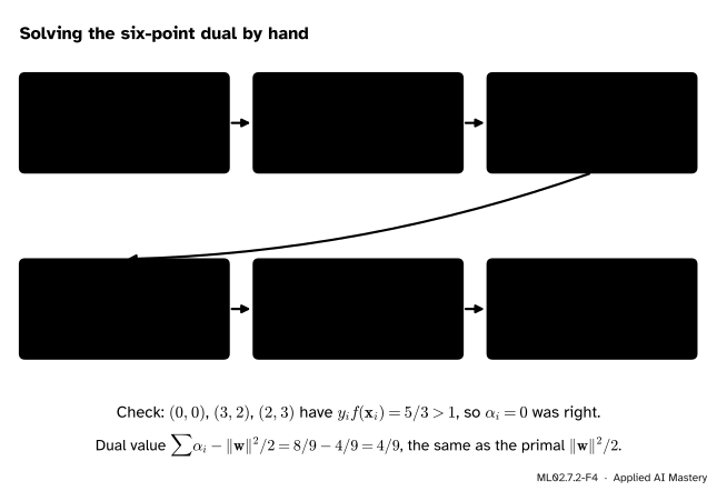
ML02.7.2-F4
The dual solved by hand once the support vectors \(\vect{x}_2\), \(\vect{x}_3\) and \(\vect{x}_4\) are guessed. Each step uses one condition.
Edges. Support vectors score exactly \(\pm 1\). For \({(1, 0)}\) and \({(0, 1)}\) the scores are \({w_1 + b = -1}\) and \({w_2 + b = -1}\), so \({w_1 = w_2}\), which forces \({\alpha_2 = \alpha_3}\). Call the common value \(a\). Then \({\alpha_4 = 2a}\) and \({\vect{w} = (4a - a,\ 4a - a) = (3a, 3a)}\), and \({b = -1 - 3a}\). For \({(2, 2)}\) the score is \(+1\):
So \({\vect{\alpha} = (0,\ \tfrac{2}{9},\ \tfrac{2}{9},\ \tfrac{4}{9},\ 0,\ 0)}\), \({\vect{w} = (\tfrac{2}{3}, \tfrac{2}{3})}\) and \({b = -1 - \tfrac{2}{3} = -\tfrac{5}{3}}\), the street of lesson 1.
Check the guess. All weights are at least \(0\), and the three points with weight \(0\) have \({y_i f(\vect{x}_i) = 5/3 > 1}\). Every condition holds, so this is the optimum.
Both values agree.\({\sum_i \alpha_i = 8/9}\) and \({\norm{\vect{w}}^2 = 8/9}\). The dual value is \({8/9 - \tfrac{1}{2} \cdot 8/9 = 4/9}\) and the primal value is \({\tfrac{1}{2} \cdot 8/9 = 4/9}\).
Code
The dual is a quadratic objective with one equation and six bounds, which scipy.optimize.minimize handles with the SLSQP method. SciPy minimises, so we minimise minus the dual objective. The matrix \({Q_{ij} = y_i y_j\, \vect{x}_i \cdot \vect{x}_j}\) holds every dot product the problem needs.
import numpy as npfrom scipy.optimize import minimizeX = np.array([[0, 0], [1, 0], [0, 1], [2, 2], [3, 2], [2, 3]], dtype=float)y = np.array([-1, -1, -1, 1, 1, 1], dtype=float)K = X @ X.T # the Gram matrix of dot productsQ = np.outer(y, y) * Kdef neg_dual(a):return0.5* a @ Q @ a - a.sum()def neg_dual_grad(a):return Q @ a -1.0result = minimize(neg_dual, np.zeros(len(y)), jac=neg_dual_grad, method="SLSQP", bounds=[(0, None)] *len(y), constraints=[{"type": "eq", "fun": lambda a: a @ y, "jac": lambda a: y}], options={"ftol": 1e-12})alpha = result.xprint("alpha:", np.round(alpha, 4))
alpha: [0. 0.2222 0.2222 0.4444 0. 0. ]
From \(\vect{\alpha}\) back to the street: \(\vect{w}\) from stationarity, \(b\) from the support vectors (averaged, which is safer with rounding), then the checks of the worked example.
w = [0.6667 0.6667]  b = -1.6667
support vectors: [[1.0, 0.0], [0.0, 1.0], [2.0, 2.0]]
y * score: [1.6667 1.     1.     1.     1.6667 1.6667]
dual value: 0.4444   primal value: 0.4444
The last hidden check is complementary slackness: every product \({\alpha_i [y_i f(\vect{x}_i) - 1]}\) is zero. Now scikit-learn. Its dual_coef_ stores \({y_i \alpha_i}\) for the support vectors only.
The solver never looked at a coordinate: it used only the Gram matrix. That observation is the whole of the next module.
Explore
In the margin explorer of lesson 3, choose Six points and Hard margin. The read-out lists each support vector with its weight: \(0.222\), \(0.222\) and \(0.444\). Drag \({(3, 2)}\) towards the street. Its weight stays \(0\) until it reaches an edge; push it into the street and it becomes a support vector, the weights change and the street moves.
Pitfalls
ML02.7.2-F5
Wrong beside right. The formula \({b = y_s - \vect{w} \cdot \vect{x}_s}\) holds only at a support vector. Used at \({(0, 0)}\) it shifts the street onto two training points.
“Any training point gives the bias.”
The equation \({y_s(\vect{w} \cdot \vect{x}_s + b) = 1}\) holds only on the edges of the street, that is, for points with \({\alpha_s > 0}\). Solvers average it over the support vectors (ESL 12.2.1 does the same) because the \(\alpha_i\) come out with rounding errors.
“The weights \(\alpha_i\) can be negative for class \(-1\).”
Every \(\alpha_i\) is at least \(0\). The sign of a point’s contribution to \(\vect{w}\) comes from its label: the term is \({\alpha_i y_i \vect{x}_i}\). scikit-learn’s dual_coef_ stores the product \({y_i \alpha_i}\), which is why it shows negative numbers.
“Points far from the street help to fix it, as in least squares.”
In least squares or logistic regression every point pulls on the answer. In the hard-margin SVM only the support vectors do. That makes the answer robust to points far away, and sensitive to the few points near the boundary, including a single mislabelled one: lesson 3 deals with that.
Check yourself
Recall
1. Write the hard-margin primal problem.
Show answer
Minimise \({\tfrac{1}{2}\norm{\vect{w}}^2}\) over \(\vect{w}\) and \(b\) subject to \({y_i (\vect{w} \cdot \vect{x}_i + b) \ge 1}\) for every \(i\).
2. What do the two stationarity conditions of the Lagrangian say?
Show answer
\({\vect{w} = \sum_i \alpha_i y_i \vect{x}_i}\) (from the derivative with respect to \(\vect{w}\)) and \({\sum_i \alpha_i y_i = 0}\) (from the derivative with respect to \(b\)).
3. State complementary slackness and what it implies for a point off the street.
Show answer
\({\alpha_i [y_i(\vect{w} \cdot \vect{x}_i + b) - 1] = 0}\) for every \(i\). Off the street the bracket is positive, so \({\alpha_i = 0}\).
4. How is \(b\) recovered once \(\vect{\alpha}\) is known?
Show answer
Compute \(\vect{w}\) from the first stationarity condition, then \({b = y_s - \vect{w} \cdot \vect{x}_s}\) for any support vector \(\vect{x}_s\), or the average over all of them.
5. Through what quantity do the data enter the dual problem?
Show answer
Only through the dot products \({\vect{x}_i \cdot \vect{x}_j}\), the entries of the Gram matrix.
Exercises
1.★ For the six points, use \({\vect{w} = \sum_i \alpha_i y_i \vect{x}_i}\) with \({\vect{\alpha} = (0, \tfrac{2}{9}, \tfrac{2}{9}, \tfrac{4}{9}, 0, 0)}\) to compute the score of the new point \({(1, 2)}\) in the dual form \({\sum_i \alpha_i y_i\, \vect{x}_i \cdot \vect{x} + b}\), and say which class is predicted.
Show solution
The dot products of \({(1, 2)}\) with the support vectors are \({(1, 0) \cdot (1, 2) = 1}\), \({(0, 1) \cdot (1, 2) = 2}\) and \({(2, 2) \cdot (1, 2) = 6}\). So
The score is positive, so class \(+1\). It agrees with \({\vect{w} \cdot (1, 2) + b = \tfrac{2}{3} + \tfrac{4}{3} - \tfrac{5}{3} = \tfrac{1}{3}}\). The point lies inside the street, since \({\abs{f} < 1}\).
2.★★ One feature: class \(-1\) at \({x = 0}\) and class \(+1\) at \({x = 2}\). Write the dual problem, solve it by hand and recover \(w\) and \(b\).
Show solution
The dot products are \({0 \cdot 0 = 0}\), \({0 \cdot 2 = 0}\) and \({2 \cdot 2 = 4}\), so only the product \({x_2 x_2 = 4}\) survives and the dual objective is \({\alpha_1 + \alpha_2 - \tfrac{1}{2} \cdot 4\,\alpha_2^2}\). Balance gives \({\alpha_1 = \alpha_2 =: a}\), so maximise \({2a - 2a^2}\). Its derivative \({2 - 4a}\) is zero at \({a = \tfrac{1}{2}}\). Then \({w = \alpha_2 \cdot 1 \cdot 2 - \alpha_1 \cdot 1 \cdot 0 = 1}\), and from the support vector \({x = 2}\): \({b = 1 - 1 \cdot 2 = -1}\). The boundary is \({x = 1}\), the width \({2 / w = 2}\), and \({\sum \alpha_i = 1 = w^2}\) as the identity in the “go deeper” note says.
3.★★★ Show that weak duality holds for the hard-margin problem: for any feasible \((\vect{w}, b)\) and any \({\vect{\alpha} \ge 0}\) with \({\sum_i \alpha_i y_i = 0}\), the dual objective is at most \({\tfrac{1}{2}\norm{\vect{w}}^2}\).
Show solution
Let \(D(\vect{\alpha})\) be the dual objective. By the derivation in the formal statement, \(D(\vect{\alpha})\) is the value of \(L\) at \({\vect{w}_\alpha = \sum_i \alpha_i y_i \vect{x}_i}\), which is where the convex function \({L(\cdot, b, \vect{\alpha})}\) has zero gradient, so it is the smallest value of \(L\) over all weight vectors (and \(L\) does not depend on \(b\) when \({\sum_i \alpha_i y_i = 0}\)). Hence
for the feasible \((\vect{w}, b)\). In \(L\), each bracket \({y_i(\vect{w} \cdot \vect{x}_i + b) - 1}\) is at least \(0\) by feasibility and each \({\alpha_i \ge 0}\), so the subtracted sum is at least \(0\) and \({L(\vect{w}, b, \vect{\alpha}) \le \tfrac{1}{2}\norm{\vect{w}}^2}\). Chaining the two inequalities proves the claim.
Summary card
Only the support vectors carry weight.
ML02.7.2-F1
The weights build \(\vect{w}\).
Primal. Minimise \({\tfrac{1}{2}\norm{\vect{w}}^2}\) with every \({y_i f(\vect{x}_i) \ge 1}\).
Dual. Maximise \({\sum_i \alpha_i - \tfrac{1}{2}\norm{\vect{w}}^2}\) over \({\alpha_i \ge 0}\) with \({\sum_i \alpha_i y_i = 0}\), and \(\vect{w}\) as above; the data enter only as \({\vect{x}_i \cdot \vect{x}_j}\).
Slackness.\({\alpha_i > 0}\) only on the edges; \({b = y_s - \vect{w} \cdot \vect{x}_s}\).
Six points.\({\vect{\alpha} = (0, \tfrac{2}{9}, \tfrac{2}{9}, \tfrac{4}{9}, 0, 0)}\), both optimal values \(4/9\).
Sources and next steps
Sources. Each was opened and checked against this lesson on 15 November 2026.
Trevor Hastie, Robert Tibshirani and Jerome Friedman, The Elements of Statistical Learning, 2nd edition, Section 4.5.2: the primal (4.48), the Lagrangian (4.49), the stationarity conditions (4.50) and (4.51), the Wolfe dual (4.52) with \({\alpha_i \ge 0}\), and the condition (4.53) from which a point off the slab gets \({\alpha_i = 0}\) and \(\beta_0\) is found from any support point. Section 12.2.1 notes that the average over the support points is used for numerical stability.
Kilian Weinberger, Lecture 9: SVM, Cornell CS4780, Fall 2018: the problem as “find the simplest hyperplane”, with smaller \({\vect{w}\T\vect{w}}\), that keeps every point at a score of at least \(1\).
scikit-learn 1.9 User Guide, Section 1.4.7.1: the dual with \({Q_{ij} = y_i y_j K(\vect{x}_i, \vect{x}_j)}\), and dual_coef_ holding the product \({y_i \alpha_i}\).
SciPy 1.18 documentation, minimize(method='SLSQP'): sequential least squares programming with bounds and with equality and inequality constraints.
Next.ML02.7.3 Soft margins and the hinge loss adds two points that no line can separate and lets the rules bend at a price \(C\). Module ML02.8 replaces the dot products by kernels; M08.7 and M08.8 give the theory of Lagrange multipliers and duality in full.