Build a K-class classifier out of binary ones. One-vs-rest trains K and takes the largest score, one-vs-one trains K(K-1)/2 and votes, and output codes add spare bits that correct mistakes. Plus SAMME, the multi-class AdaBoost, and its extra ln(K-1).
ML02.10.2L2 Intermediate25 minIn review (what this means)
The maths and code on this page are checked by automated tests on every change, but an independent reader has not signed it off yet. Spot a mistake or a confusing step? Tell us.
Build one-vs-rest and one-vs-one classifiers from any binary learner, and find the regions where their binary answers abstain, overlap or tie.
Count the classifiers and the training work of each reduction, and explain why SVC uses one-vs-one.
Decode an error-correcting output code by Hamming distance and state how many wrong bits it can correct.
State SAMME’s learner weight and explain the extra ln(K - 1) term.
The question
An SVM answers one question: which side of the street is this point on? Softmax regression had a score for every class, but the SVM has only the one. How do we turn a learner that can only say yes or no into one that names one of \(K\) classes, and what do we lose on the way?
From the last lesson
1. What is the gradient of the cross-entropy loss with respect to \(\vect{w}_k\)?
Show answer
\({(p_k - y_k)\,\vect{x}}\): the probability of class \(k\) minus its one-hot label, times the input.
2. Why do micro precision and accuracy agree in a single-label problem?
Show answer
Every mistake is one false positive and one false negative, so the pooled counts give precision and recall both equal to the number correct over \(n\).
Intuition
There are two natural ways to ask yes-or-no questions about \(K\) classes. One-vs-rest asks one question per class: “is it class \(k\), or one of the others?” One-vs-one holds a duel for every pair: “class \(j\) or class \(k\)?”, and lets the duels vote.
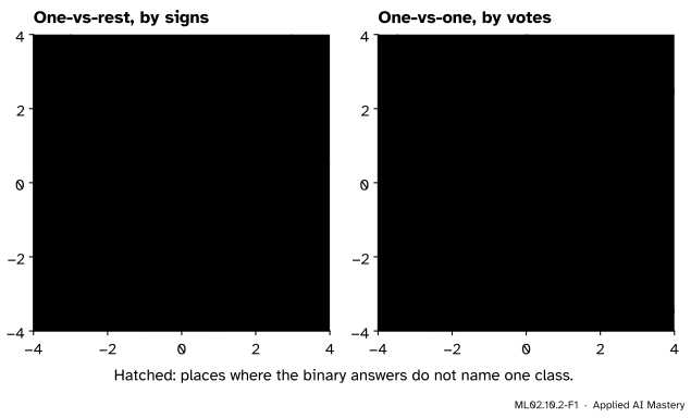
Both work most of the time. The interesting part is where they fail: places where the binary answers do not add up to one class.
ML02.10.2-F1
The three clusters with hand-made linear rules. Left: three one-vs-rest rules leave a hole that no rule claims and corners that two rules claim. Right: three pairwise duels leave a small triangle where the duels go round in a circle and every class gets one vote.
each positive for its own class. For one-vs-one, \({g_{12} = -x_1}\) says class 1 when positive and class 2 when negative; \({g_{13} = 0.5 - x_1 - x_2}\) decides between 1 and 3; and \({g_{23} = x_1 - x_2 - 1.5}\) between 2 and 3. All twelve points are classified correctly by every rule. The trouble is only in the empty space between the clusters, where new points may land.
Build it up
Step 1. One-vs-rest by signs. Train \(K\) binary classifiers; classifier \(k\) sees class \(k\) as positive and all other classes as negative. A new point may get no “yes” at all, or several.
Step 2. One-vs-rest by the largest score. Use the real-valued scores, not only their signs, and pick the class whose classifier is most confident: \({\argmax_k f_k(\vect{x})}\). This is what ISL Section 9.4.2 prescribes for SVMs. Every point now gets exactly one class.
Step 3. One-vs-one by votes. Train one classifier per pair of classes, each only on the examples of its two classes. Each duel gives a vote; the class with the most votes wins (ISL 9.4.1).
Step 4. Breaking a tie. With three classes the duels can form a cycle: 2 beats 1, 1 beats 3, 3 beats 2. scikit-learn then adds up each class’s confidences over its duels and picks the largest sum.
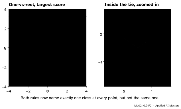
ML02.10.2-F2
Resolving the ambiguity. Left: comparing scores gives one-vs-rest a full partition with straight borders. Right: inside the tie, the summed confidences split the triangle three ways.
The formal statement
NoteTwo reductions
Given a binary learner that returns a real score (positive for the positive class):
One-vs-rest trains \(K\) scorers \(f_1, \dots, f_K\), where \(f_k\) separates class \(k\) from all the others, and predicts \({\hat{y} = \argmax_k f_k(\vect{x})}\).
One-vs-one trains \({K(K - 1)/2}\) scorers \(g_{jk}\) for \({j < k}\), each on the examples of classes \(j\) and \(k\) only, and predicts the class with the most pairwise wins. scikit-learn breaks a tie in votes by the summed confidences.
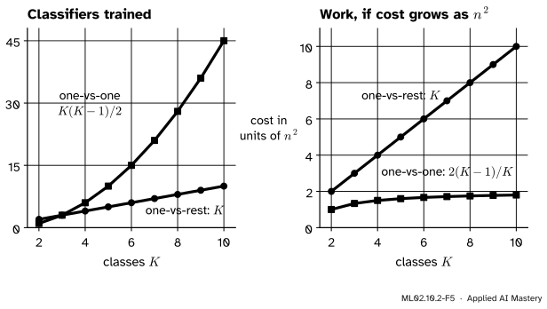
What each one costs. Suppose \(n\) examples split evenly over \(K\) classes. One-vs-rest trains \(K\) classifiers, each on all \(n\) examples. One-vs-one trains \({K(K - 1)/2}\) classifiers, each on the \({2n/K}\) examples of its pair. Count the total training work for a learner whose cost grows like \(n^2\):
The second line expands the square to \({4n^2/K^2}\) and cancels one \(K\) and the \(2\). For ten classes, one-vs-rest does \({10\,n^2}\) of work and one-vs-one \({1.8\,n^2}\): many more classifiers, much less work.
ML02.10.2-F5
More classifiers, smaller problems. Kernel SVM training grows between \(n^2\) and \(n^3\), so many small problems are cheaper than a few big ones.
The quadratic-programming solver behind scikit-learn’s SVC scales between \({n^2}\) and \({n^3}\) (User Guide 1.4.4). The User Guide recommends one-vs-one for exactly such kernel methods, which scale badly with the number of examples (1.12.1.3), and SVC and NuSVC always train one-vs-one internally (1.4.1.1). For a linear model whose cost grows like \(n\), the saving all but disappears: one-vs-one sees \({(K - 1)\,n}\) examples in all against \({K n}\). LinearSVC uses one-vs-rest.
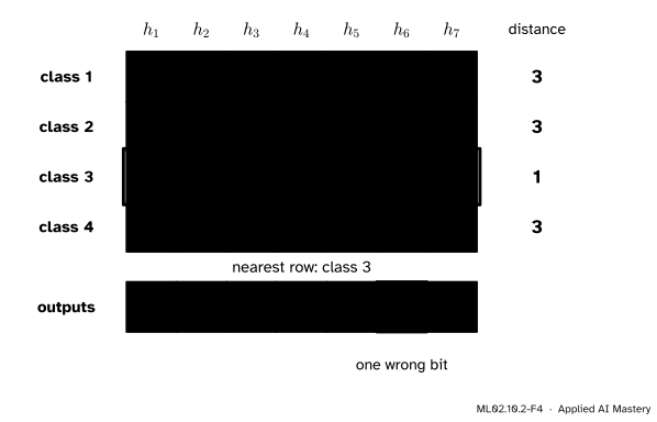
Error-correcting output codes. Write a code matrix with one row per class and one column per binary classifier. Classifier \(h_j\) learns to output the bit in column \(j\) for every example of each class. To predict, run all the classifiers and pick the class whose row, its codeword, is nearest to the output word in Hamming distance, the number of differing bits.
If any two codewords differ in at least \(d\) places, up to \({\lfloor (d - 1)/2 \rfloor}\) wrong bits still leave the true codeword nearest (Dietterich and Bakiri, Section 1). One-vs-rest is the code whose rows have a single 1; two such rows differ in only 2 places, so it corrects nothing. With three classes there are only three useful columns, which is just one-vs-rest again. From four classes on there is room for spare bits.
ML02.10.2-F4
The exhaustive code for four classes has seven columns, and every two rows differ in exactly 4 places. One wrong output still decodes to the right class.
SAMME, the multi-class AdaBoost. Instead of reducing to binary problems, Zhu, Rosset, Zou and Hastie keep a multi-class weak learner (a tree that names one of \(K\) classes) and change one line of AdaBoost (ML02.3.2). The learner weight becomes
and misclassified examples have their weights multiplied by \(e^{\alpha_m}\). Why the extra term? Guessing at random among \(K\) classes is wrong \({(K - 1)/K}\) of the time. The weight is positive exactly when
so a learner only has to beat random guessing, not the much harder target \({\epsilon_m < 1/2}\). For \({K = 2}\) the extra term is \({\ln 1 = 0}\) and SAMME is AdaBoost with every \(\alpha_m\) doubled, which gives the same sign and the same classifier.
Go deeper: where ln(K - 1) comes from: the multi-class exponential loss
Code class \(c\) as a vector \(\vect{y}\) of length \(K\) with \({y_c = 1}\) and every other entry \({-1/(K - 1)}\), and let the model be a vector \(\vect{f}(\vect{x})\) with entries summing to zero. Zhu and colleagues use the loss \({\exp(-\tfrac{1}{K}\,\vect{y} \cdot \vect{f})}\). A weak learner \(T\) that names class \(T(\vect{x})\) is coded the same way as a vector \(\vect{g}\), and each stage adds \({\beta\,\vect{g}}\).
If \({T(\vect{x}) = c}\), the two vectors are equal, and
with \(\alpha_m\) exactly the SAMME weight above; that is Lemma 1 of the paper. For \({K = 2}\) the factor is \({1/2}\) and \({\beta = \tfrac{1}{2}\ln\tfrac{1 - \epsilon}{\epsilon}}\), the AdaBoost weight of ML02.3.2. The weight update \({e^{-\beta\,\vect{y}\cdot\vect{g}/K}}\) is \({e^{-\beta/(K - 1)}}\) for a correct example and \({e^{\beta/(K - 1)^2}}\) for a wrong one, whose ratio is \(e^{\alpha_m}\): after renormalising, only the wrong examples grow.
Worked example
One new point through both reductions. Take \({\vect{x} = (0.2,\ -0.8)}\), in the middle of the three clusters.
One-vs-rest.\({f_1 = -2 - 0.4 + 0.8 = -1.6}\), \({f_2 = -2 + 0.4 + 0.8 = -0.8}\) and \({f_3 = -0.8 - 0.5 = -1.3}\). No score is positive, so by signs no class claims the point. The largest score is \({f_2 = -0.8}\): class 2.
One-vs-one.\({g_{12} = -0.2}\), so 2 beats 1. \({g_{13} = 0.5 - 0.2 + 0.8 = 1.1}\), so 1 beats 3. \({g_{23} = 0.2 + 0.8 - 1.5 = -0.5}\), so 3 beats 2. Every class has one vote. Sum each class’s confidences, counting a duel’s score as positive for the class it favours:
from \({-0.2 + 1.1}\), \({0.2 - 0.5}\) and \({-1.1 + 0.5}\).
Class 1 wins the tie.
ML02.10.2-F3
The same point, two reductions, two different answers: class 2 from one-vs-rest, class 1 from one-vs-one.
Neither answer is wrong; the point is far from every cluster and the binary rules disagree about it. The reductions agree on the twelve training points and differ only in the regions that the first figure hatched.
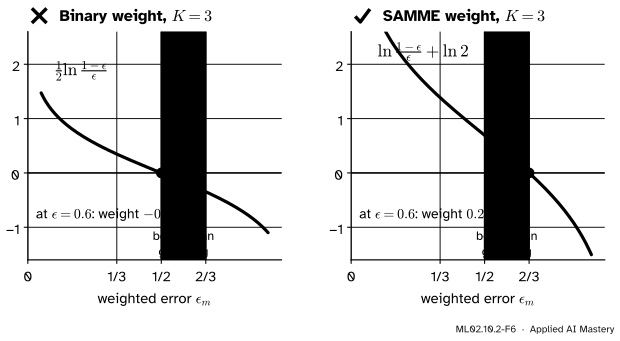
A SAMME weight. On iris, three classes of equal size, a stump can name only two classes, so it misclassifies at least one class: a weighted error of \({1/3}\) at the first round. SAMME gives it \({\alpha = \ln 2 + \ln 2 = \ln 4 = 1.386}\). The binary formula would give \({\tfrac{1}{2}\ln 2 = 0.347}\), and a stump with error \({0.6}\) would get a negative weight.
Code
From scratch on iris: one-vs-rest and one-vs-one built around LinearSVC, which is used only as a binary learner here.
import warningsimport numpy as npfrom sklearn.base import clonefrom sklearn.datasets import load_irisfrom sklearn.model_selection import train_test_splitfrom sklearn.preprocessing import StandardScalerfrom sklearn.svm import LinearSVCwarnings.filterwarnings("ignore")iris = load_iris()Xtr, Xte, ytr, yte = train_test_split(iris.data, iris.target, test_size=0.4, random_state=0, stratify=iris.target)scaler = StandardScaler().fit(Xtr)Xtr, Xte = scaler.transform(Xtr), scaler.transform(Xte)base = LinearSVC(random_state=0)# one-vs-rest: K scorers, then the largest scoreF = np.column_stack([clone(base).fit(Xtr, ytr == k).decision_function(Xte) for k inrange(3)])claims = np.bincount((F >0).sum(axis=1), minlength=4)ovr = F.argmax(axis=1)# one-vs-one: a duel per pair, votes, and summed confidence for tiesvotes, conf = np.zeros((len(Xte), 3)), np.zeros((len(Xte), 3))for i, j in [(0, 1), (0, 2), (1, 2)]: pair = (ytr == i) | (ytr == j) d = clone(base).fit(Xtr[pair], ytr[pair] == j).decision_function(Xte) # positive: j votes[d >0, j] +=1 votes[d <=0, i] +=1 conf[:, j] += d conf[:, i] -= dovo = (votes + conf / (3* (np.abs(conf) +1))).argmax(axis=1) # scikit-learn's tie-breakprint("test flowers claimed by 0, 1, 2, 3 one-vs-rest classifiers:", claims)print("one-vs-rest correct:", int((ovr == yte).sum()), "of 60; one-vs-one correct:",int((ovo == yte).sum()), "of 60")
test flowers claimed by 0, 1, 2, 3 one-vs-rest classifiers: [12 42  6  0]
one-vs-rest correct: 57 of 60;  one-vs-one correct: 58 of 60
Twelve of the sixty test flowers fall in the “no class” hole and six in an overlap, yet the largest score still gets 57 right. The library versions do exactly the same.
from sklearn.multiclass import OneVsOneClassifier, OneVsRestClassifier, OutputCodeClassifierlib_ovr = OneVsRestClassifier(base).fit(Xtr, ytr)lib_ovo = OneVsOneClassifier(base).fit(Xtr, ytr)ecoc = OutputCodeClassifier(base, code_size=2, random_state=0).fit(Xtr, ytr)print("same as ours:", np.array_equal(lib_ovr.predict(Xte), ovr), np.array_equal(lib_ovo.predict(Xte), ovo))print("output code book (one row per class):\n", ecoc.code_book_.astype(int))print("output codes correct:", int((ecoc.predict(Xte) == yte).sum()), "of 60")
same as ours: True True
output code book (one row per class):
 [[ 1  1  1  1 -1  1]
 [-1  1  1 -1  1  1]
 [ 1  1 -1 -1 -1  1]]
output codes correct: 52 of 60
code_size=2 asks for \({2K = 6}\) random columns. Two of them came out the same for all three classes, so those classifiers learn nothing, and the code does worse than one-vs-rest. With three classes there is no room for a good code, as the formal section showed.
Last, SAMME inside scikit-learn’s AdaBoostClassifier, checked against the formula.
Three classes of points with a logistic-regression classifier per class, per pair, or all trained together. Switch between one-vs-rest, one-vs-one and softmax, and drag the points (or move them with the sliders) to see the regions redraw.
Things to try:
In one-vs-rest with binary answers only, the read-out gives the share of the drawing that no class or several classes claim. Press resolve to one class: the largest score fills the hatched places, and the hatching fades to mark where the signs alone were unclear.
In one-vs-one, the three duel lines start out meeting in one point, so there is no tie. Set the penalty to its smallest value and move a point of class 3 down among the others, for example to \({(1.5, -2)}\): the duel lines no longer meet in one point, and a hatched region of ties, about 2.5% of the drawing, opens between them.
In softmax, there is never a hole or a tie: one model, one score per class. Drag the points about: the three borders always meet in one point, because where \({z_1 = z_2}\) and \({z_2 = z_3}\) hold, \({z_1 = z_3}\) holds too.
Pitfalls
ML02.10.2-F6
Wrong beside right, for three classes. A learner with weighted error \({0.6}\) beats random guessing, which errs \({2/3}\) of the time. The binary formula gives it a negative weight; SAMME gives it a small positive one.
“Multi-class AdaBoost is binary AdaBoost run on a multi-class learner.”
Then any stage with error above \({1/2}\) gets a negative weight, and the reweighting runs the wrong way. Zhu and colleagues show this stalling binary AdaBoost on a three-class problem. The \({\ln(K - 1)}\) term moves the break-even point to the error of random guessing, \({(K - 1)/K}\).
“One-vs-rest scores can be compared as they are.”
Each one-vs-rest classifier is trained alone, and nothing puts their scores on one scale. Multiply \(f_3\) by 3 and it makes exactly the same yes-or-no decisions, yet the largest-score regions move. Scale the features, use the same learner and settings for every class, or use calibrated probabilities (ML04.7) before comparing.
“One-vs-one must be slow, it trains so many classifiers.”
It trains more classifiers but on smaller sets. For a learner whose cost grows faster than linearly in \(n\), such as a kernel SVM, the total work is less than for one-vs-rest. Count the work, not the classifiers.
Check yourself
Recall
1. How many binary classifiers do one-vs-rest and one-vs-one train for \(K\) classes?
Show answer
One-vs-rest trains \(K\); one-vs-one trains \({K(K - 1)/2}\), one per pair.
2. In one-vs-rest by signs, what two kinds of ambiguous region can appear?
Show answer
Regions where no classifier says yes, and regions where two or more do. Taking the largest score removes both.
3. Why does SVC train one-vs-one internally?
Show answer
Kernel SVM training grows between \(n^2\) and \(n^3\), and one-vs-one trains each classifier on only two classes’ examples, so its total work is smaller than one-vs-rest’s.
4. A code has minimum Hamming distance 4 between codewords. How many wrong bits can it correct?
Show answer
\({\lfloor (4 - 1)/2 \rfloor = 1}\).
5. Write SAMME’s learner weight. When is it positive?
Show answer
\({\alpha_m = \ln\frac{1 - \epsilon_m}{\epsilon_m} + \ln(K - 1)}\). It is positive when \({\epsilon_m < (K - 1)/K}\), that is, when the learner beats random guessing.
Exercises
1.★ Classify \({\vect{x} = (-2, 3)}\) with the one-vs-rest rules of this lesson, first by signs and then by the largest score.
Show solution
\({f_1 = -2 + 4 - 3 = -1}\), \({f_2 = -2 - 4 - 3 = -9}\), \({f_3 = 3 - 0.5 = 2.5}\). Only \(f_3\) is positive, so both methods say class 3.
2.★★ A problem has \({K = 10}\) classes of equal size and \({n = 10{,}000}\) examples. Count the classifiers and the total number of training examples they see under one-vs-rest and one-vs-one, and compare the work for a learner whose cost grows like \(n^2\).
Show solution
One-vs-rest: 10 classifiers on \({10{,}000}\) examples each, \({100{,}000}\) in all. One-vs-one: 45 classifiers on \({2{,}000}\) examples each, \({90{,}000}\) in all, which is \({(K - 1)\,n}\). With cost proportional to \(n^2\), one-vs-rest does \({10 \times 10{,}000^2 = 10^9}\) units and one-vs-one \({45 \times 2{,}000^2 = 1.8 \times 10^8}\), less than a fifth as much, matching \({2(K - 1)/K = 1.8}\) against \(10\).
3.★★★ With the four-class code of the figure, a point gives the outputs \({1011001}\). Decode it. Then show that two wrong bits can leave the decoder unable to choose.
Show solution
Distances: to class 1 (\({1111111}\)) there are 3 differences; to class 2 (\({0000111}\)), 5; to class 3 (\({0011001}\)), 1 (the first bit); to class 4 (\({0101010}\)), 5. So it decodes to class 3, the first bit having been wrong. For two errors, start from class 3 and flip bits 2 and 6, which gives \({0111011}\). Its distance to class 3 is 2, and to class 1 (bits 1 and 5) and to class 4 (bits 3 and 7) it is 2 as well: a three-way tie. Since every two codewords differ in 4 places, two errors can reach the halfway point between codewords, which is why only \({\lfloor 3/2 \rfloor = 1}\) error is guaranteed to be corrected.
Summary card
Binary learners make \(K\) classes by voting in teams: one-vs-rest, one-vs-one, or a code.
Sources. Each was opened and checked against this lesson on 15 November 2026.
Gareth James, Daniela Witten, Trevor Hastie and Robert Tibshirani, An Introduction to Statistical Learning, 2nd edition, Section 9.4: one-versus-one with \({\binom{K}{2}}\) SVMs and a tally of votes (9.4.1), and one-versus-all with \(K\) SVMs and the class of largest score (9.4.2).
scikit-learn 1.9 User Guide, Section 1.12.1: OneVsRestClassifier with n_classes classifiers, OneVsOneClassifier with \({K(K - 1)/2}\) classifiers, voting and the tie-break by summed confidence, the remark that one-vs-one suits kernel methods that scale badly with n_samples (1.12.1.3), and OutputCodeClassifier with its random code book. Section 1.4: SVC and NuSVC train one-vs-one and LinearSVC one-vs-rest (1.4.1.1), and the solver scales between \({n^2}\) and \({n^3}\) (1.4.4).
Thomas G. Dietterich and Ghulum Bakiri, Solving Multiclass Learning Problems via Error-Correcting Output Codes, Journal of Artificial Intelligence Research 2, 263 to 286 (1995). Section 1: minimum distance \(d\) corrects \({\lfloor (d - 1)/2 \rfloor}\) errors, and one-per-class codes correct none. Section 2.3: only three useful columns for three classes, and the seven-column exhaustive code of distance 4 for four.
Ji Zhu, Saharon Rosset, Hui Zou and Trevor Hastie, Multi-class AdaBoost, preprint of 12 January 2006, published in Statistics and Its Interface in 2009. Algorithm 2 with the weight (1), the condition that each learner beat random guessing, the coding (2) and loss (3), and Lemma 1 with (13).