Let every class keep its own covariance and the boundary bends into an ellipse, a parabola or a hyperbola. Derive quadratic discriminant analysis, fit it to iris by hand and in NumPy, count what it costs in parameters, and use shrinkage when a class has too few points.
ML02.9.3L2 Intermediate25 minIn review (what this means)
The maths and code on this page are checked by automated tests on every change, but an independent reader has not signed it off yet. Spot a mistake or a confusing step? Tell us.
Derive the quadratic discriminant function and explain why its boundaries are conics.
Compute the QDA scores of a point by hand and implement QDA from scratch, checked against scikit-learn.
Count the covariance parameters of LDA and QDA and explain why a class with fewer than d + 1 points has a singular covariance.
Use shrinkage towards a multiple of the identity as a bias-variance choice, and choose its strength on validation data.
The question
LDA forced the twelve points’ two very different clouds, a leaning cigar and an upright oval, into one shared shape. What happens if each class keeps the shape it really has? And if more freedom fits better, why not always take it?
From the last lesson
1. Which assumption makes the discriminant functions of LDA linear?
Show answer
All classes share one covariance matrix, so \({\vect{x}\T\mat{\Sigma}^{-1}\vect{x}}\) and \({\ln\det\mat{\Sigma}}\) are the same for every class and drop out.
2. How is the pooled covariance estimated?
Show answer
Add each class’s scatter about its own mean and divide by \(n\) (or by \({n - K}\)); equivalently, average the class covariances with weights \({n_k/n}\).
Intuition
Give each class its own ellipse. Now the two clouds differ in shape as well as in place, and the line where they are equally high is no longer straight: it bends round the tighter cloud and away from the wider one.
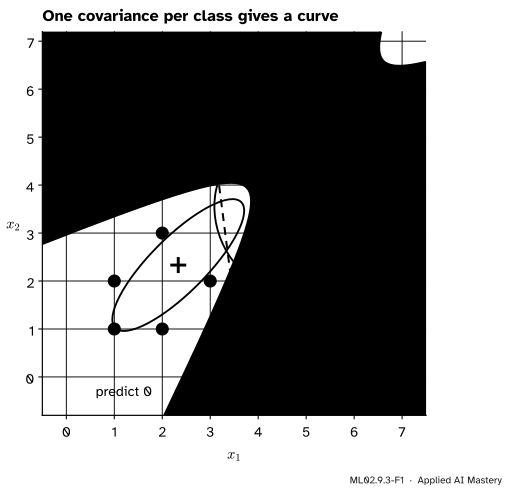
ML02.9.3-F1
Quadratic discriminant analysis on the twelve points. Each class keeps its own covariance, and the boundary curves round class 0’s narrow cloud. Only \({(5, 5)}\) is now misclassified.
This is quadratic discriminant analysis (QDA). The point \({(2, 5)}\), which LDA put in class 0, is now correctly in class 1: it lies across the narrow axis of class 0’s cigar, so class 0 finds it unlikely, while class 1’s rounder cloud does not mind it.
Build it up
Step 1. Keep the term that cancelled. With a covariance \(\mat{\Sigma}_k\) per class, the term \({-\tfrac12\vect{x}\T\mat{\Sigma}_k^{-1}\vect{x}}\) differs from class to class, so it stays in each score.
Step 2. Keep the log-determinant too.\({-\tfrac12\ln\det\mat{\Sigma}_k}\) also differs. It is larger for a tighter class: a narrow cloud has a high peak, so near its centre it beats a wide cloud that happens to be centred nearby.
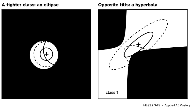
Step 3. The boundary is a curve of degree two. Subtract two scores. The result has terms in \(x_1^2\), \(x_2^2\) and \({x_1x_2}\), terms in \(x_1\) and \(x_2\), and a constant. Setting it to zero gives a conic: an ellipse, a parabola or a hyperbola (or, in special cases, a pair of lines).
ML02.9.3-F2
Two kinds of conic boundary. A class much tighter than the other is closed in by an ellipse; two classes that lean in opposite directions are split by a hyperbola.
The formal statement
NoteDefinition: quadratic discriminant analysis
Model each class as \({N(\vect{\mu}_k, \mat{\Sigma}_k)}\) with its own covariance, and priors \(\pi_k\). The quadratic discriminant function is
and QDA predicts the class with the largest \(\delta_k(\vect{x})\). Each class is fitted on its own, by the maximum-likelihood mean and covariance of ML02.9.1.
Derivation. The log of \({\pi_k N(\vect{x};\, \vect{\mu}_k, \mat{\Sigma}_k)}\) in \(d\) dimensions is \(\delta_k(\vect{x})\) minus \({\tfrac d2\ln(2\pi)}\). Only that constant is shared by all classes, so only it is dropped. That is all: QDA is the generative recipe of ML02.9.1, scored in logs.
Why the boundary is a conic. For two classes write \({\mat{P}_k = \mat{\Sigma}_k^{-1}}\) and expand each quadratic form as in ML02.9.2:
The boundary \({\vect{x}\T\mat{Q}\vect{x} + \vect{w}\T\vect{x} + b = 0}\) is a conic, and the signs of the two eigenvalues of \(\mat{Q}\) say which: the same sign gives an ellipse, opposite signs a hyperbola, and one zero a parabola. When \({\mat{\Sigma}_1 = \mat{\Sigma}_0}\), \({\mat{Q} = \mat{0}}\) and we are back to LDA’s line. For the twelve points the eigenvalues of \(\mat{Q}\) are \({-0.18}\) and \({1.26}\): a hyperbola, as in the anchor figure.
What the freedom costs. A covariance matrix in \(d\) dimensions is symmetric, so it has \({d(d + 1)/2}\) free numbers. LDA estimates one, QDA one per class:
Model
Covariance parameters
\(d = 4\), \(K = 3\)
\(d = 13\), \(K = 3\)
LDA
\({d(d + 1)/2}\)
10
91
QDA
\({K\,d(d + 1)/2}\)
30
273
The last two columns are iris and wine. More parameters means more variance: each \(\hat{\mat{\Sigma}}_k\) is estimated from one class’s points alone.
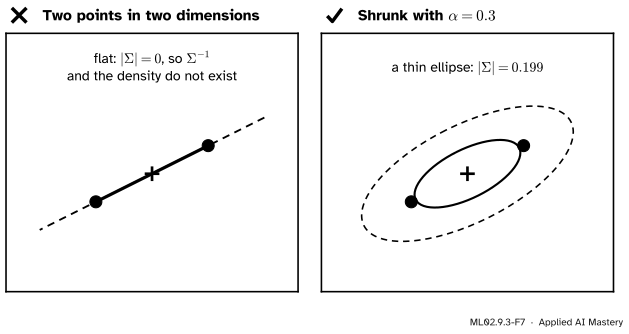
Too few points: a singular covariance. The deviations \({\vect{x}_i - \hat{\vect{\mu}}_k}\) of a class add up to zero, so at most \({n_k - 1}\) of them are independent, and \({\hat{\mat{\Sigma}}_k}\), a sum of their outer products, has rank at most \({n_k - 1}\). If \({n_k < d + 1}\) the rank is below \(d\): \({\det\hat{\mat{\Sigma}}_k = 0}\), the inverse does not exist, and QDA cannot score that class at all.
Shrinkage. The remedy is to pull the estimate towards something simpler that is always invertible. Friedman’s regularised discriminant analysis (ESL section 4.3.1) shrinks each class covariance towards the pooled one, and the pooled one towards a multiple of the identity:
scikit-learn’s shrinkage parameter uses the second kind, with the weight written the other way round: \({(1 - \alpha)\hat{\mat{\Sigma}} + \alpha\,\tau\mat{I}}\), where \({\tau = \operatorname{tr}\hat{\mat{\Sigma}}/d}\) is the average variance. Every eigenvalue becomes \({(1 - \alpha)\lambda_i + \alpha\tau}\), which is positive for any \({\alpha > 0}\), so the shrunk matrix is always invertible. Shrinkage adds bias (the truth is rarely a multiple of the identity) and removes variance (fewer numbers are left free to fit noise), and the right amount depends on how much data there is.
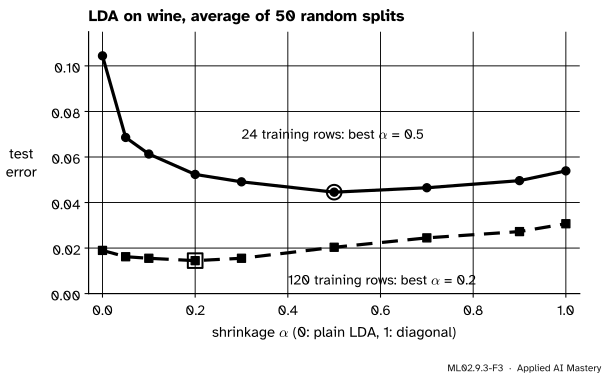
ML02.9.3-F3
Shrinkage as a bias-variance dial. With 24 training rows, strong shrinkage helps a lot; with 120, a little helps and too much hurts.
Worked example
Classify the iris flower with petal length 5.6 cm and width 1.4 cm, using QDA on the two petal features of all 150 flowers.
Setosa is far away, so compare versicolor (\(k = 1\)) and virginica (\(k = 2\)). Each class has 50 flowers, so \({\ln\pi_k = \ln(1/3) = -1.099}\) for both. The fitted means and covariances are
The determinant terms.\({\det\hat{\mat{\Sigma}}_1}\)\({= 0.2164 \cdot 0.0383 - 0.0716^2}\)\({= 0.00316}\) and \({\det\hat{\mat{\Sigma}}_2 = 0.01978}\). So \({-\tfrac12\ln\det}\) is 2.878 for versicolor and 1.962 for virginica: versicolor’s cloud is tighter, so it starts ahead.
The distance terms. The deviation from versicolor’s mean is \({(1.34, 0.074)}\). Inverting the 2 by 2 matrix as in ML02.9.2,
Versicolor’s cloud is thin and leans with correlation 0.79, and this flower sits off its axis. For virginica the deviation is \({(0.048, -0.626)}\) and the same formula gives \({\Delta_2^2 = 6.07}\).
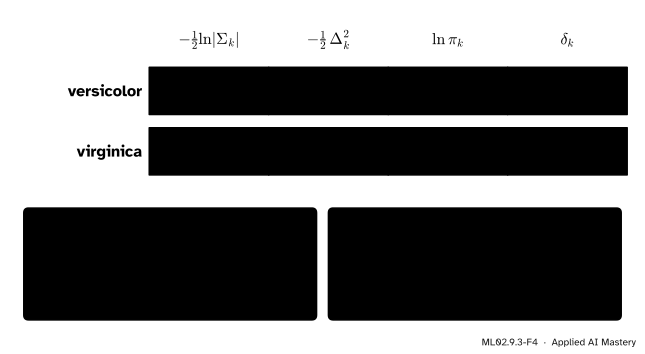
ML02.9.3-F4
The worked example as a table. Virginica’s larger cloud loses on the determinant but wins easily on distance.
Decide.\({\delta_1 = 2.878 - 8.825 - 1.099 = -7.046}\) and \({\delta_2 = 1.962 - 3.034 - 1.099 = -2.171}\). Virginica wins by almost 5 in log units, a posterior of about 0.99, and the flower is indeed a virginica. LDA, which gives both classes the pooled covariance, measures squared distances of 11.65 and 12.93 and wrongly picks versicolor.
Code
QDA from scratch, checked on the twelve points and then on the iris petals against scikit-learn.
import numpy as npfrom sklearn.datasets import load_irisfrom sklearn.discriminant_analysis import LinearDiscriminantAnalysis, QuadraticDiscriminantAnalysisdef qda_fit(X, y): classes = np.unique(y) prior = np.array([np.mean(y == k) for k in classes]) means = np.array([X[y == k].mean(axis=0) for k in classes]) covs = np.array([np.cov(X[y == k].T, bias=True) for k in classes])return prior, means, covsdef qda_scores(X, prior, means, covs): out = []for p, m, S inzip(prior, means, covs): V = X - m m2 = np.einsum("ij,ij->i", V @ np.linalg.inv(S), V) # squared Mahalanobis distances out.append(-0.5* np.log(np.linalg.det(S)) -0.5* m2 + np.log(p))return np.array(out).Tdef softmax(s): e = np.exp(s - s.max(axis=1, keepdims=True))return e / e.sum(axis=1, keepdims=True)X12 = np.array([(1, 1), (2, 1), (1, 2), (2, 3), (3, 2), (5, 5), (4, 1), (5, 2), (5, 3), (4, 4), (2, 5), (6, 5)], dtype=float)y12 = np.array([0] *6+ [1] *6)prior, means, covs = qda_fit(X12, y12)Q =-0.5* (np.linalg.inv(covs[1]) - np.linalg.inv(covs[0]))print("twelve points: right", (qda_scores(X12, prior, means, covs).argmax(axis=1) == y12).sum(),"of 12; eigenvalues of Q:", np.linalg.eigvalsh(Q).round(3))X, y = load_iris(return_X_y=True)X = X[:, 2:] # petal length and widthfit = qda_fit(X, y)ours = softmax(qda_scores(X, *fit))library = QuadraticDiscriminantAnalysis().fit(X, y)print("iris: largest difference from scikit-learn:", f"{np.abs(ours - library.predict_proba(X)).max():.1e}")print("training right: QDA", (ours.argmax(axis=1) == y).sum(), "LDA", (LinearDiscriminantAnalysis().fit(X, y).predict(X) == y).sum(), "of 150")flower = np.array([[5.6, 1.4]])print("delta at (5.6, 1.4):", qda_scores(flower, *fit).round(3), " P(virginica):",round(softmax(qda_scores(flower, *fit))[0, 2], 3))
twelve points: right 11 of 12; eigenvalues of Q: [-0.177  1.263]
iris: largest difference from scikit-learn: 6.7e-16
training right: QDA 147 LDA 144 of 150
delta at (5.6, 1.4): [[-292.017   -7.045   -2.171]]  P(virginica): 0.992
ML02.9.3-F5
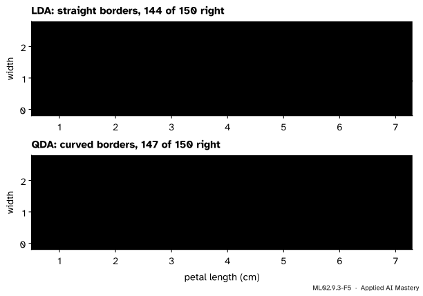
LDA and QDA on the iris petals. QDA’s versicolor region follows the thin, tilted versicolor cloud, which moves the ringed flower into virginica.
Now shrinkage on load_wine, with 13 features, after standardising. With only 36 training rows, the classes have 12, 14 and 10 rows, and two of them are below \({d + 1 = 14}\).
from sklearn.datasets import load_winefrom sklearn.model_selection import train_test_splitfrom sklearn.preprocessing import StandardScalerXw, yw = load_wine(return_X_y=True)X_tr, X_te, y_tr, y_te = train_test_split(Xw, yw, train_size=36, random_state=0, stratify=yw)scaler = StandardScaler().fit(X_tr)A, B = scaler.transform(X_tr), scaler.transform(X_te)print("rows per class:", np.bincount(y_tr), " ranks of the class covariances:", [int(np.linalg.matrix_rank(np.cov(A[y_tr == k].T, bias=True))) for k inrange(3)])for model in (QuadraticDiscriminantAnalysis(), QuadraticDiscriminantAnalysis(reg_param=0.5), QuadraticDiscriminantAnalysis(solver="eigen", shrinkage="auto")):try:print(model, "test accuracy", round(model.fit(A, y_tr).score(B, y_te), 3))except np.linalg.LinAlgError:print(model, "cannot be fitted: a class covariance is singular")def shrink(S, alpha):return (1- alpha) * S + alpha * np.trace(S) /len(S) * np.eye(len(S))Sigma =sum(np.mean(y_tr == k) * np.cov(A[y_tr == k].T, bias=True) for k inrange(3))lsqr = LinearDiscriminantAnalysis(solver="lsqr", shrinkage=0.3).fit(A, y_tr)print("from-scratch shrinkage matches scikit-learn:", np.allclose(shrink(Sigma, 0.3), lsqr.covariance_))
rows per class: [12 14 10]  ranks of the class covariances: [11, 13, 9]
QuadraticDiscriminantAnalysis() cannot be fitted: a class covariance is singular
QuadraticDiscriminantAnalysis(reg_param=0.5) cannot be fitted: a class covariance is singular
QuadraticDiscriminantAnalysis(shrinkage='auto', solver='eigen') test accuracy 0.958
from-scratch shrinkage matches scikit-learn: True
The plain QDA cannot be fitted, and reg_param does not rescue it: with the default 'svd' solver scikit-learn regularises only the directions the class’s points span, and still refuses a class with \({n_k \le d}\) rows. solver="eigen" with shrinkage works. Finally the curve of the figure above: LDA with each shrinkage \(\alpha\), averaged over 50 random splits, for 24 and 120 training rows.
24 rows: error at alpha 0 0.104, best 0.045 at alpha 0.5, at alpha 1 0.054
120 rows: error at alpha 0 0.019, best 0.014 at alpha 0.2, at alpha 1 0.031
With 24 rows, plain LDA errs on 10.4% of the test wines and the best shrinkage, \({\alpha = 0.5}\), cuts that to 4.5%. With 120 rows the best is small, \({\alpha = 0.2}\) in this run (0.1 and 0.3 make only three more mistakes over all 50 splits, so a different machine’s arithmetic could pick one of them), and full shrinkage (every feature given the same spread and no correlations) is clearly worse. In practice, choose \(\alpha\) by cross-validation, or let shrinkage="auto" pick it by the Ledoit and Wolf formula.
Explore
ML02.9-X1
Ellipse explorer
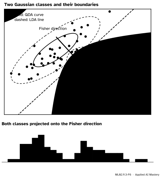
Pick a class, then drag its centre or the handle on its ellipse, or use the sliders, to move, stretch and turn it. Switch Shared covariance on and off to compare the LDA line with the QDA curve, and add a third class. Beneath the plane, the classes are projected onto Fisher’s direction.
Three things to try. Make the two ellipses the same shape and see the QDA curve straighten into the LDA line. Make one class small and round inside a wide one, and watch the curve close into an ellipse. Then turn the two ellipses in opposite directions and read the training accuracy of LDA and QDA in the read-out: how far apart can you push them?
Pitfalls
ML02.9.3-F7
Wrong beside right. Two points in two dimensions give a covariance with no width across the line through them. Shrinkage restores a thin ellipse that can be inverted.
“QDA is more flexible than LDA, so it is always at least as good.”
More flexible means more parameters, \({K\,d(d + 1)/2}\) against \({d(d + 1)/2}\), each estimated from one class’s points. ISLR (section 4.4.3) puts it as a bias-variance trade-off: LDA tends to be the better bet with few training points, QDA with many or when the classes clearly differ in shape. On wine with 36 training rows, plain QDA cannot even be fitted.
“A class with a handful of points still has a covariance matrix.”
It has one, but with \({n_k \le d}\) points it is singular: the points span at most \({n_k - 1}\) directions, and across the others the fitted cloud has zero width. Its inverse and its density do not exist. Shrink it, pool it with the other classes (LDA), or drop features.
“Shrinkage towards the identity is the same whatever the units of the features.”
A multiple of the identity treats every feature as equally spread. If one feature is in grams and another in kilograms, shrinkage pulls them very unequally. Standardise first, as in the code above; shrinkage="auto" in scikit-learn standardises internally for the same reason.
Check yourself
Recall
1. Which two terms of the QDA score do not cancel between classes, though they did in LDA?
Show answer
\({-\tfrac12\vect{x}\T\mat{\Sigma}_k^{-1}\vect{x}}\) (inside the quadratic form) and \({-\tfrac12\ln\det\mat{\Sigma}_k}\).
2. What shapes can a two-class QDA boundary take, and what decides it?
Show answer
A conic: an ellipse, a parabola or a hyperbola (or degenerate cases such as a pair of lines). The signs of the eigenvalues of \({\mat{Q} = -\tfrac12(\mat{\Sigma}_1^{-1} - \mat{\Sigma}_0^{-1})}\) decide.
3. How many covariance parameters do LDA and QDA estimate?
Show answer
LDA \({d(d + 1)/2}\); QDA \({K\,d(d + 1)/2}\).
4. Why is the covariance of a class with \({n_k \le d}\) points singular?
Show answer
Its deviations from the class mean sum to zero, so they span at most \({n_k - 1 < d}\) directions, and the covariance has rank at most \({n_k - 1}\).
5. What does scikit-learn’s shrinkage\(\alpha\) do to a covariance estimate?
Show answer
It replaces \(\hat{\mat{\Sigma}}\) by \({(1 - \alpha)\hat{\mat{\Sigma}} + \alpha\,(\operatorname{tr}\hat{\mat{\Sigma}}/d)\,\mat{I}}\): 0 keeps the estimate, 1 replaces it by a multiple of the identity.
Exercises
1.★ Count the covariance parameters of LDA and QDA for load_breast_cancer (\({d = 30}\), \({K = 2}\)), and the smallest class size for which QDA’s class covariance can be invertible.
Show solution
\({d(d + 1)/2 = 30 \cdot 31/2 = 465}\) for LDA, and \({2 \cdot 465 = 930}\) for QDA. Each class needs at least \({d + 1 = 31}\) points for its covariance to have full rank.
2.★★ Two classes in one dimension have equal priors, \({\mu_0 = 0}\), \({\sigma_0 = 1}\) and \({\mu_1 = 0}\), \({\sigma_1 = 2}\). Find the QDA boundary. Where does LDA put it?
Show solution
In one dimension \({\delta_k = -\ln\sigma_k - x^2/(2\sigma_k^2)}\) (dropping the equal priors). Setting \({\delta_1 = \delta_0}\):
So QDA predicts class 0 for \({\abs{x} < 1.36}\) and class 1 outside: the wider class wins in both tails, the one-dimensional version of an ellipse closing round the tighter class. LDA gives both classes the same variance; with equal means its two discriminants are then identical everywhere, so it cannot tell the classes apart at all.
3.★★★ Show that for any \({\alpha > 0}\) the matrix \({(1 - \alpha)\hat{\mat{\Sigma}} + \alpha\tau\mat{I}}\), with \({\tau = \operatorname{tr}\hat{\mat{\Sigma}}/d > 0}\) and \(\hat{\mat{\Sigma}}\) positive semidefinite, is positive definite. What are its eigenvectors?
Show solution
Let \({\hat{\mat{\Sigma}}\vect{u} = \lambda\vect{u}}\) with \({\lambda \ge 0}\). Then
so the shrunk matrix has the same eigenvectors, and eigenvalues \({(1 - \alpha)\lambda + \alpha\tau}\). For \({0 < \alpha \le 1}\) the first part is at least 0 and the second is positive, so every eigenvalue is positive and the matrix is positive definite, hence invertible. The ellipses keep their directions; the long axes shrink towards the average width and the short ones grow towards it.
Summary card
One covariance per class: the quadratic terms stay, and the boundary is a conic.
Boundary:\({\vect{x}\T\mat{Q}\vect{x} + \vect{w}\T\vect{x} + b = 0}\), a conic.
Cost:\({K\,d(d + 1)/2}\) covariance parameters; singular when \({n_k \le d}\).
Shrinkage:\({(1 - \alpha)\hat{\mat{\Sigma}} + \alpha\tau\mat{I}}\); choose \(\alpha\) on validation data.
Sources and next steps
Sources. Each was opened and checked against this lesson on 15 November 2026.
T. Hastie, R. Tibshirani and J. Friedman, The Elements of Statistical Learning, 2nd edition, corrected 12th printing (2017). Section 4.3: the quadratic discriminant functions, equation (4.12), and the dramatic increase in parameters when \(p\) is large. Section 4.3.1: Friedman’s regularised discriminant analysis, with \({\hat\Sigma_k(\alpha) = \alpha\hat\Sigma_k + (1 - \alpha)\hat\Sigma}\) (4.13) and \({\hat\Sigma(\gamma) = \gamma\hat\Sigma + (1 - \gamma)\hat\sigma^2 I}\) (4.14), chosen on validation data.
G. James, D. Witten, T. Hastie and R. Tibshirani, An Introduction to Statistical Learning, 2nd edition (with R), section 4.4.3: the QDA discriminant (4.28), the count of \({Kp(p + 1)/2}\) covariance parameters, and the bias-variance argument for choosing between LDA and QDA.
scikit-learn, Linear and Quadratic Discriminant Analysis, User Guide section 1.2: shrinkage with 'lsqr' or 'eigen' (only 'eigen' for QDA), shrinkage='auto' by the Ledoit and Wolf lemma; and the QuadraticDiscriminantAnalysis reference for reg_param, which transforms each class’s scalings as \({(1 - r)S^2 + r}\), and for the maximum-likelihood (biased) class covariances.