A decision tree asks one yes-or-no question about one feature at a time until it reaches an answer. Read a tree both as a diagram and as rectangles of the feature plane, walk a new point to its leaf, and see why a leaf predicts the majority class or the mean.
ML02.1.1L2 Intermediate25 minIn review (what this means)
The maths and code on this page are checked by automated tests on every change, but an independent reader has not signed it off yet. Spot a mistake or a confusing step? Tell us.
Name the parts of a decision tree: root, internal node, branch, leaf and depth.
Predict the class of a new point by walking a tree from its root to a leaf.
Draw the axis-aligned rectangles that a tree cuts the feature plane into, and read a tree back off them.
Show that the majority class minimises the errors in a leaf and the mean minimises its squared error.
The question
A loan officer decides with a short list of questions: is the income above some amount? If not, is there a guarantor? Twelve labelled points in the plane can be sorted the same way, by asking one yes-or-no question about one feature at a time. What does such a list of questions look like as a picture, and what does it do to the plane?
Intuition
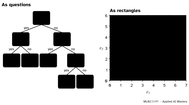
This course’s twelve points sit in the plane with two features, \(x_1\) and \(x_2\). Six belong to class 0 (blue circles) and six to class 1 (sky-blue squares). Here is one way to sort them, drawn twice.
ML02.1.1-F1
The same tree, read two ways. On the left, each box asks one question and each leaf gives an answer, with the class counts of the training points that reach it. On the right, each question is a cut through the plane, and each leaf is a rectangle.
A decision tree starts at the top with one question, such as “is \(x_1 \le 3.5\)?”. The answer sends a point down one of two paths, where it meets another question, and so on, until it reaches an answer. Every question looks at a single feature and compares it with a single number.
Read as a picture of the plane, each question is a straight cut parallel to an axis. The cuts nest: the second question on the left only cuts the left part of the plane. When the questions run out, the plane has been cut into rectangles, and every point in a rectangle gets the same answer.
Build it up
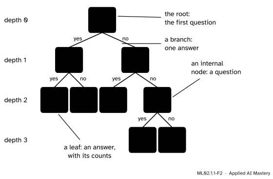
Step 1. Name the parts. The first question is the root. Every box that asks a question is an internal node, and every box that gives an answer is a leaf. The two lines leaving a question are its branches: by convention the left one is “yes” and the right one is “no”. The depth of a node is the number of questions above it, so the root has depth 0, and the depth of the tree is the depth of its deepest leaf.
ML02.1.1-F2
The parts of a tree. This one has four questions, five leaves and depth 3.
Step 2. One question. Ask only the root question, \(x_1 \le 3.5\). The plane splits into a left half with 5 points of class 0 and 1 of class 1, and a right half with 1 and 5. If each half answers with its more common class, the tree gets 10 of the 12 points right. A tree with a single question is called a stump.
Step 3. Ask again on each side. The one class-1 point on the left is \((2, 5)\), high up. The question \(x_2 \le 4\) cuts it off, and the left half becomes two pure rectangles. On the right, the question \(x_2 \le 4.5\) separates four class-1 points below from a mixed pair above, and one last question, \(x_1 \le 5.5\), splits that pair. Now every rectangle holds points of one class only.
Step 4. Count. Each question turns one leaf into two, so it adds exactly one leaf. A tree with \(k\) questions has \(k + 1\) leaves: here four questions and five leaves.
The next two lessons explain how a computer finds these questions. This lesson is about reading a tree once you have one.
The formal statement
NoteDefinition: a binary decision tree
Every internal node holds a test\(x_j \le s\) on one feature \(j\) against a threshold\(s\). A point that passes the test goes to the left child; a point that fails goes to the right. Every leaf holds a prediction. The leaves cut the feature space into regions \(R_1, \dots, R_J\), one per leaf, and the tree predicts
where \(\cmodel{v_m}\) is the value stored in leaf \(m\).
Each region is a box. The points that reach a leaf are those that pass or fail every test on the way down. Each test keeps one side of a cut: \(x_j \le s\) or \(x_j > s\). Keeping one side of several such cuts keeps an interval of each feature, so the region is a rectangle in the plane (a box in \(d\) dimensions), with sides parallel to the axes. Every point goes down exactly one path, so the regions do not overlap and together they cover the whole space.
The best answer for a class leaf is the majority. Say \(n_m\) training points reach leaf \(m\), and \(n_{mk}\) of them are in class \(k\). If the leaf answers \(k\), it gets the other \({n_m - n_{mk}}\) points wrong. That count is smallest when \(n_{mk}\) is largest, so the leaf should answer with its most common class. The share \(n_{mk}/n_m\) is the leaf’s estimate of the probability of class \(k\) there.
The best answer for a number leaf is the mean. For a regression tree the leaf answers a number \(v\), and its squared error on its points is
\[
S(v) = \sum_{i \in R_m} (y_i - v)^2 .
\]
Differentiate with respect to \(v\) and set the result to zero:
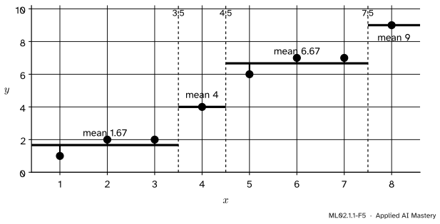
The second derivative is \(2 n_m > 0\), so this is a minimum. A regression tree therefore predicts the mean target of the training points in each leaf, and on one feature it draws a staircase.
ML02.1.1-F5
A regression tree with three questions on the eight-point set of this course. Each leaf predicts the mean of its points, so the prediction is a staircase. The purple bars are the errors that the mean makes as small as possible.
Worked example
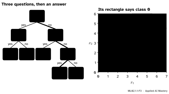
Classify the new point \((5.2, 4.8)\) with the tree of the twelve points.
Start at the root and answer one question at a time.
Is \(x_1 \le 3.5\)? Here \(x_1 = 5.2\), so no: go right.
Is \(x_2 \le 4.5\)? Here \(x_2 = 4.8\), so no: go right.
Is \(x_1 \le 5.5\)? Here \(x_1 = 5.2\), so yes: go left.
That box is a leaf holding one training point, \((5, 5)\), of class 0. The answer is class 0.
ML02.1.1-F3
The walk, both ways. Three answers (no, no, yes) lead to a leaf. In the plane, the same answers pick out the rectangle that holds the point.
The second panel shows the same thing without any questions: the star lies in the rectangle \(3.5 < x_1 \le 5.5\), \(x_2 > 4.5\), which the tree labels class 0. Notice that the star’s other near neighbours, \((6, 5)\) and \((4, 4)\), are both class 1, yet the tree says class 0, because of a single training point at \((5, 5)\). A tree grown until every leaf is pure follows single points like this one. Lesson 4 returns to that.
A second point, \((2, 4.5)\): \(x_1 = 2 \le 3.5\), yes; \(x_2 = 4.5 \le 4\), no. It lands in the leaf that holds \((2, 5)\), and the answer is class 1. Two questions were enough, because that leaf has depth 2. Walking a tree costs at most one comparison per level, which is why a prediction is fast.
Code
A tree is nested if statements. Here is the tree of the twelve points written by hand.
import numpy as nppoints = np.array([(1, 1), (2, 1), (1, 2), (2, 3), (3, 2), (5, 5), (4, 1), (5, 2), (5, 3), (4, 4), (2, 5), (6, 5)], dtype=float)labels = np.array([0] *6+ [1] *6)def by_hand(x1, x2):if x1 <=3.5:return0if x2 <=4else1if x2 <=4.5:return1return0if x1 <=5.5else1hand = np.array([by_hand(*p) for p in points])print("right on the training points:", int((hand == labels).sum()), "of", len(labels))print("(5.2, 4.8) ->", by_hand(5.2, 4.8), " (2, 4.5) ->", by_hand(2, 4.5))
right on the training points: 12 of 12
(5.2, 4.8) -> 0   (2, 4.5) -> 1
Writing every tree as code would be tedious, so store it as data instead: each node is either a leaf with an answer or a question with two children. One short loop walks any such tree.
The regression tree with three questions predicts \(1.67\), \(4\), \(6.67\) and \(9\): the means of the four pieces in the staircase figure.
Explore
This module’s interactive, the tree grower, lives in lesson 3. There you press a button to add one question at a time and watch the rectangles appear beside the growing diagram.
Pitfalls
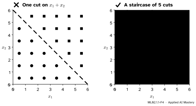
ML02.1.1-F4
Wrong beside right. The boundary the data need is a slanted line, but no single question of a tree can draw it, because each question uses one feature. A tree builds a staircase of cuts instead, stepping down beside the diagonal (dotted).
“A tree can ask about a mix of features, such as \(x_1 + x_2 \le 6\).”
A standard tree cannot: each test looks at one feature. A slanted boundary costs many questions and is still only a staircase. Where the true boundary is a straight line at an angle, a linear model such as logistic regression (ML01.6) needs two weights and a bias where a tree needs a whole staircase. Where the boundary really is made of boxes, the tree wins.
“A pure leaf is a sure answer.”
A leaf’s counts are counts of training points. The leaf \(3.5 < x_1 \le 5.5\), \(x_2 > 4.5\) is pure because it holds a single point. One example is weak evidence, and lesson 4 shows that trees which chase single points predict badly on new data.
“Points on a threshold are ambiguous.”
They are not. The test is \(x_j \le s\), so a point exactly on the cut goes left, every time. In practice thresholds are placed halfway between training values, as lesson 3 explains, so no training point sits on one.
Check yourself
Recall
1. What is the difference between an internal node and a leaf?
Show answer
An internal node asks a question \(x_j \le s\) and has two children. A leaf asks nothing and gives the prediction.
2. What shape is the region of a leaf, and why?
Show answer
A rectangle (a box in higher dimensions) with sides parallel to the axes. Each test on the path keeps one side of a cut on one feature, so the region is an interval in each feature.
3. A tree has seven questions. How many leaves does it have?
Show answer
Eight. Each question turns one leaf into two, so it adds one leaf to the single leaf you start with.
4. What does a leaf predict in a classification tree, and in a regression tree?
Show answer
The majority class of the training points in the leaf, and the mean of their targets.
5. Which class does the tree of the twelve points give to \((3, 4.5)\)?
Show answer
Class 1: \(x_1 = 3 \le 3.5\), yes; \(x_2 = 4.5 \le 4\), no; the leaf of \((2, 5)\) says class 1.
Exercises
1.★ Walk the points \((4, 4.6)\), \((6, 4.6)\) and \((0.5, 0.5)\) down the tree of the twelve points and give each answer.
2.★★ A regression leaf holds the targets 3, 5 and 10. Find the value that minimises the squared error, and show that it beats the median, 5.
Show solution
The mean is \({(3 + 5 + 10)/3} = 6\). Its squared error is \({9 + 1 + 16} = 26\). The median 5 gives \({4 + 0 + 25} = 29\), which is larger. The derivation in the formal statement says the mean is the minimum, so any other value, the median included, does worse.
3.★★★ Write the five leaf regions of the tree of the twelve points as inequalities, and check that every point of the plane lies in exactly one of them.
Show solution
Following each path from the root:
\(x_1 \le 3.5\) and \(x_2 \le 4\): class 0.
\(x_1 \le 3.5\) and \(x_2 > 4\): class 1.
\(x_1 > 3.5\) and \(x_2 \le 4.5\): class 1.
\(3.5 < x_1 \le 5.5\) and \(x_2 > 4.5\): class 0.
\(x_1 > 5.5\) and \(x_2 > 4.5\): class 1.
Every point has either \(x_1 \le 3.5\) or \(x_1 > 3.5\), and not both. In the first case it has either \(x_2 \le 4\) or \(x_2 > 4\), which picks one of the first two regions. In the second case, \(x_2 \le 4.5\) picks the third region; otherwise \(x_1 \le 5.5\) or \(x_1 > 5.5\) picks the fourth or the fifth. At each step exactly one choice holds, so exactly one region contains the point.
Summary card
A decision tree is a list of one-feature questions, and a partition of space into boxes.
ML02.1.1-F1
Questions on the left, rectangles on the right.
Test. Each internal node asks \(x_j \le s\): yes goes left, no goes right.
Regions. The leaves cut the space into axis-aligned boxes \(R_1, \dots, R_J\).
Leaf values. Majority class for classification; mean target for regression.
Size.\(k\) questions give \(k + 1\) leaves; a prediction costs one comparison per level.
Sources and next steps
Sources. Each was opened and checked against this lesson on 15 November 2026.
G. James, D. Witten, T. Hastie, R. Tibshirani and J. Taylor, An Introduction to Statistical Learning, 2nd edition (free PDF from the authors). Section 8.1 describes trees as boxes in the predictor space with the mean (regression) or most common class (classification) as the prediction; Section 8.1.3 shows a tree losing to a linear model on a slanted boundary (Figure 8.7); Section 8.1.4 lists the advantages, including that trees are easy to explain, and the drawback that they are non-robust.
T. Hastie, R. Tibshirani and J. Friedman, The Elements of Statistical Learning, 2nd edition, 12th printing. Section 9.2.2 writes the tree as a constant on each region, equation (9.10), and shows that the best constant under squared error is the average, equation (9.11).
scikit-learn developers, User Guide, Section 1.10: Decision Trees (version 1.9). The classes DecisionTreeClassifier and DecisionTreeRegressor, the test \(x_j \le t_m\) that sends a point left, and export_text.