A test that finds 90% of cases and wrongly flags 10% of healthy people says you are positive. The chance you have the condition is 1 in 12. Count it out on a grid of 1,000 people and see why the base rate decides the answer.
Turn a base rate and the two rates of a test into whole-number counts on a grid of 1,000 people, and read the posterior off the grid.
Compute P(condition | positive) with Bayes’ rule and show that it matches the count.
Describe how the posterior climbs with the base rate, from 1/12 at a base rate of 1% to 9/10 at 50%.
Recognise base-rate neglect and the prosecutor’s fallacy as the same swap of P(E | H) for P(H | E), and connect the posterior to the precision of a classifier.
In review. The maths and code on this page are checked by automated tests on every change, but an independent reader has not signed it off yet. Spot a mistake or a confusing step? Tell us.
The question
One person in a hundred has a certain condition. A test finds 90% of the people who have it, and wrongly flags 10% of the people who do not. You take the test and it comes back positive. Many people guess that you now have about a 90% chance of having the condition. The true answer is about 8%. Where did the other 82 points go?
From the last lesson
1. State Bayes’ rule and name its four parts.
Show answer
\({\Prob(H \mid E)} = {\Prob(E \mid H)\,\Prob(H) / \Prob(E)}\): the posterior equals the likelihood times the prior, divided by the evidence.
2. In the inbox, \({\Prob(\text{free} \mid \text{spam}) = 0.6}\) but \({\Prob(\text{spam} \mid \text{free}) = 0.8}\). Why are they different?
Show answer
They share the overlap of 24 emails but divide by different totals: 40 spam emails in one, 30 ‘free’ emails in the other.
Intuition
Probabilities such as 1%, 90% and 10% are hard to combine in your head. Counts are easy. So imagine 1,000 people and turn every rate into a number of people.
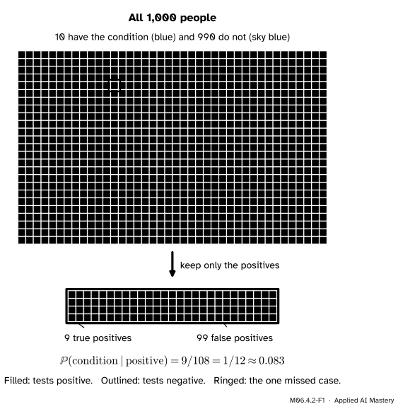
1% of 1,000 is 10 people who have the condition; the other 990 do not.
The test is positive for 90% of the 10: 9 true positives.
The test is positive for 10% of the 990: 99 false positives.
M06.4.2-F1
The test, counted on 1,000 people. A positive result puts you in the block at the bottom, and only 9 of its 108 people have the condition.
A positive result tells you one thing: you are somewhere in the block of 108 positives. Nine of them have the condition, so your chance is \({9/108 = 1/12}\), about 8%. The test is good, but the 990 healthy people outnumber the 10 sick people by 99 to 1, so even their small error rate makes far more positives than the condition does.
The share of people who have the condition before any test is called the base rate (in medicine, the prevalence). It is the prior of Bayes’ rule, and this lesson is about how much it matters.
Build it up
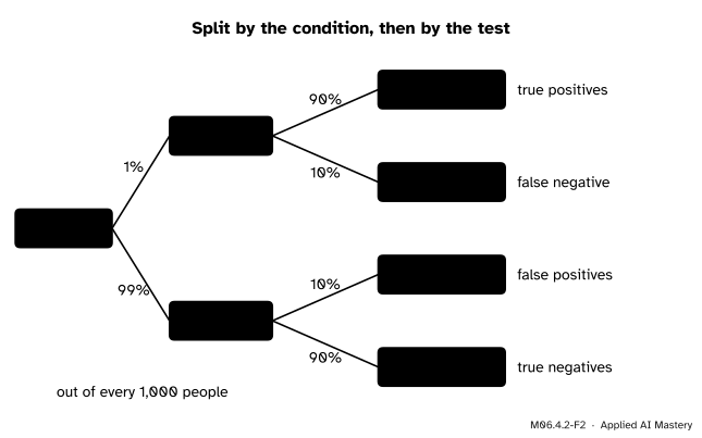
Step 1. Split by the condition. Start with 1,000 people and split them by the base rate: \({1{,}000 \times 0.01 = 10}\) have the condition and 990 do not.
Step 2. Split each group by the test. Each group meets the test at its own rate. Of the 10, \({10 \times 0.9 = 9}\) test positive and 1 is missed. Of the 990, \({990 \times 0.1 = 99}\) test positive and 891 test negative.
M06.4.2-F2
The same 1,000 people as a tree of natural frequencies: each branch carries a count of people instead of a probability.
Step 3. Keep only the positives. Your result was positive, so the two yellow leaves are the only people you could be: \({9 + 99 = 108}\) of them.
Step 4. Read the share. Of those 108, the 9 true positives have the condition: \({9/108 = 1/12}\).
Nothing in these four steps is new. Step 1 uses the prior, step 2 the two likelihoods, step 3 the law of total probability and step 4 the division in Bayes’ rule. The counts only make each step something you can see.
The formal statement
NoteBayes’ rule for a test
Write \(\pi\) for the base rate \({\Prob(D)}\), where \(D\) is “has the condition”. Write \(s\) for \({\Prob(+ \mid D)}\), the share of people with the condition who test positive, and \(f\) for \({\Prob(+ \mid D^c)}\), the share of the others who test positive. Then
This is Bayes’ rule from M06.4.1 with \(H = D\), \({E = +}\), and the evidence expanded by the law of total probability. On the grid, multiplying the whole formula by 1,000 turns each term into a count: the numerator is the true positives and the denominator is all the positives. In medicine \(s\) is called the sensitivity, and \({1 - f}\) the specificity.
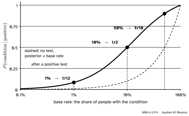
How the posterior climbs with the base rate. For the course’s test, \({s = 0.9}\) and \({f = 0.1}\). Multiply the top and bottom of the formula by 10:
at \({\pi = 0.01}\): \({0.09 / 1.08 = 1/12}\), about 8%;
at \({\pi = 0.1}\): \({0.9 / 1.8 = 1/2}\);
at \({\pi = 0.5}\): \({4.5 / 5 = 9/10}\).
M06.4.2-F4
The same test, the same positive result, three different answers. Only at a base rate of 50% does the posterior come close to the 90% that many people guess.
The 90% that many people guess is the posterior only when the base rate is 50%, that is when half of the people tested have the condition. The test multiplies the odds of having the condition by the same factor wherever you start; lesson M06.4.3 makes that exact. What it cannot do is make a rare condition common.
Go deeper: why counts help
Gerd Gigerenzer and Ulrich Hoffrage gave people problems like this one with no training. In their first study, when the numbers were stated as probabilities in the usual way, 16% of the answers followed Bayesian reasoning; when the same numbers were stated as natural frequencies (“9 of the 10 people with the condition test positive”), 46% to 50% did. A count keeps track of its own reference group. The count 99 already knows it is a count of healthy people, while the bare rate 10% hides which group it belongs to. The grid is not only a trick for beginners: it is a quick check on any answer from Bayes’ rule.
Worked example
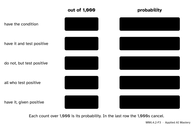
The course’s test. Base rate 1%, sensitivity 0.9, false positive rate 0.1. Find \({\Prob(D \mid +)}\) by the formula and by counting, side by side.
M06.4.2-F3
Every term of Bayes’ rule beside the count of people it stands for.
The numerator is the chance of being a true positive: \({s\pi = 0.9 \times 0.01 = 0.009}\), which is 9 people in 1,000.
The second term of the denominator is the chance of being a false positive: \({f(1 - \pi) = 0.1 \times 0.99 = 0.099}\), which is 99 people in 1,000.
The evidence is their sum, \({\Prob(+) = 0.108}\), or 108 people. The posterior is
Read the other way, \({11/12}\) of the positive results are false alarms. A positive result has still raised your chance from 1% to about 8%, more than eight times as likely as before. That is real information, and it is why a first positive result is usually followed by a second test, the subject of the next lesson.
Code
First the grid, with whole numbers of people. Fractions keep every rate exact.
from fractions import Fraction as Frpeople =1000base, sens, fpr = Fr(1, 100), Fr(9, 10), Fr(1, 10)sick = people * base # 10 people have the conditiontrue_pos = sick * sens # 9 of them test positivefalse_pos = (people - sick) * fpr # 99 of the 990 others test positiveprint(f"{sick} have it, {true_pos} true positives, {false_pos} false positives")print("P(condition | positive) =", true_pos / (true_pos + false_pos))
Now Bayes’ rule as a function of the base rate, checked against the short formula for this test.
def posterior(base, sens=Fr(9, 10), fpr=Fr(1, 10)):"""P(condition | positive) by Bayes' rule."""return sens * base / (sens * base + fpr * (1- base))for b in (Fr(1, 100), Fr(1, 10), Fr(1, 2)):print(f"base rate {float(b):.0%}: posterior {posterior(b)} (short formula {9* b / (1+8* b)})")
base rate 1%: posterior 1/12  (short formula 1/12)
base rate 10%: posterior 1/2  (short formula 1/2)
base rate 50%: posterior 9/10  (short formula 9/10)
A simulation of a million people checks the answer without using Bayes’ rule at all.
import numpy as nprng = np.random.default_rng(seed=12)n =1_000_000has_it = rng.random(n) <0.01positive = np.where(has_it, rng.random(n) <0.9, rng.random(n) <0.1)share = has_it[positive].mean()print(f"{positive.sum()} positives, of whom a share {share:.4f} have the condition (1/12 = {1/12:.4f})")
107855 positives, of whom a share 0.0828 have the condition (1/12 = 0.0833)
Think of the test as a classifier that predicts “has the condition” when it is positive. Its precision, the share of its positive predictions that are right (ML01.7.2), is exactly this posterior. scikit-learn computes it from the true labels and the predictions.
from sklearn.metrics import precision_scoreprecision = precision_score(has_it, positive)print(f"precision of the test as a classifier: {precision:.4f}")
precision of the test as a classifier: 0.0828
Explore
M06.4-X1
Frequency grid
Move the base rate and watch the blue cells thin out or spread across the grid. Press Gather the positives to collect every filled cell into one block, and compare the count with Bayes’ rule in the read-out. Try a base rate of 10% and then 50%, and then make the test perfect for healthy people by setting the false positive rate to 0.
Pitfalls
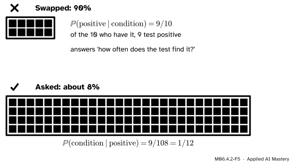
M06.4.2-F5
Wrong beside right. The 90% is a share of the 10 people with the condition. The question is about a share of the 108 people with a positive test.
“The test is 90% accurate, so a positive result means a 90% chance.”
This is base-rate neglect: answering with \({\Prob(+ \mid D) = 0.9}\), how often the test finds the condition, when the question asks for \({\Prob(D \mid +)}\). For this test the two agree only at a base rate of 50%. For a rare condition the healthy majority produces most of the positives.
“Only 1 innocent person in 1,000 would match, so the suspect is 99.9% likely to be guilty.”
This is the prosecutor’s fallacy, the same swap in a courtroom. Say a blood type found at a crime scene is shared by 1 person in 1,000, and 50,000 people could have committed the crime, each as likely as the others before the blood is tested. Besides the culprit, about 50 innocent people match. A match alone leaves the suspect as one of about 51 matching people, so the probability of guilt is about 2%, not 99.9%:
\({\Prob(\text{match} \mid \text{innocent}) = 0.001}\) is small, but \({\Prob(\text{innocent} \mid \text{match})}\) is about 0.98. Other evidence can change the prior, and so the answer; the match on its own cannot.
“My classifier has 90% recall and a 10% false positive rate, so its alarms are mostly right.”
A classifier’s precision is the posterior of this lesson, with the share of positive examples as the base rate. If 1% of the examples are positive, the classifier’s alarms are right 1 time in 12. Always read precision beside the base rate of the class it predicts (ML01.7.3).
Check yourself
Recall
1. What is a base rate, and which part of Bayes’ rule is it?
Show answer
The share of people (or cases) that have the condition before any evidence is seen. It is the prior, \({\Prob(D)}\).
2. On the grid of 1,000 people for the course’s test, how many true positives and how many false positives are there?
Show answer
9 true positives (90% of the 10 with the condition) and 99 false positives (10% of the 990 without it).
3. Why is \({\Prob(D \mid +)}\) only \({1/12}\) when the test finds 90% of cases?
Show answer
Because the condition is rare. The 990 healthy people produce 99 false positives, eleven times as many as the 9 true positives, so only 9 of the 108 positives have the condition.
4. For the course’s test, what is the posterior after a positive result at base rates of 10% and 50%?
Show answer
\({1/2}\) at 10% and \({9/10}\) at 50%, from \({9\pi / (1 + 8\pi)}\).
5. What do base-rate neglect and the prosecutor’s fallacy have in common?
Show answer
Both swap \({\Prob(E \mid H)}\) for \({\Prob(H \mid E)}\): they answer with how likely the evidence is under a hypothesis instead of how likely the hypothesis is given the evidence.
Exercises
1.★ A rarer condition affects 1 person in 1,000. The test is the same: positive for 90% of people with it and for 10% of people without. Use a grid of 10,000 people to find \({\Prob(D \mid +)}\).
Show solution
Of 10,000 people, 10 have the condition and 9 of them test positive. Of the 9,990 without it, \({9{,}990 \times 0.1 = 999}\) test positive. So \({\Prob(D \mid +)} = {9 / (9 + 999)} = {9/1{,}008} = {1/112}\), about 0.9%. The short formula agrees: \({9 \times 0.001 / (1 + 8 \times 0.001)} = {0.009 / 1.008} = {1/112}\).
2.★★ Keep the base rate at 1% and the sensitivity at 0.9, but improve the test so that only 1% of healthy people test positive. Find the posterior. Which change helps more, halving the missed cases or cutting the false positive rate?
Show solution
Use 10,000 people, so that every count is whole: 100 have the condition, 90 true positives, and \({9{,}900 \times 0.01 = 99}\) false positives. The posterior is \({90 / (90 + 99) = 90/189 = 10/21}\), about 0.476. Halving the missed cases instead (sensitivity 0.95, false positive rate still 0.1) gives 95 true positives and 990 false positives, so \({95 / 1{,}085 = 19/217}\), about 0.088, barely better than \({1/12}\). When the condition is rare, the false positives from the large healthy group decide the answer, so cutting the false positive rate helps far more.
3.★★★ For a test with sensitivity \(s\) and false positive rate \(f\), find the base rate \(\pi\) at which a positive result gives a posterior of exactly \({1/2}\). Check your answer on the course’s test.
Show solution
The posterior is \({1/2}\) when the numerator is half the denominator, that is when the true positives equal the false positives:
For \({s = 0.9}\) and \({f = 0.1}\) this gives \({\pi = 0.1 / 1.0 = 0.1}\), matching the 10% row of this lesson. Below that base rate, most positives are false alarms.
Summary card
A positive result puts you among the positives, and the base rate decides who they are.
M06.4.2-F1
9 of 108 positives: 1 in 12.
Count it. Of 1,000 people: 10 have it, 9 true positives, 99 false positives.
Bayes’ rule for a test.\({\Prob(D \mid +)} = {s\pi / (s\pi + f(1 - \pi))}\).
The course’s test.\({9\pi/(1 + 8\pi)}\): \({1/12}\) at 1%, \({1/2}\) at 10%, \({9/10}\) at 50%.
The slip. Do not answer \({\Prob(H \mid E)}\) with \({\Prob(E \mid H)}\).
Sources and next steps
Sources. Each was opened and checked against this lesson on 12 November 2026.
Jeremy Orloff and Jonathan Bloom, Reading 3: Conditional probability, independence and Bayes’ theorem, MIT OpenCourseWare 18.05, Spring 2022. Section 7.1, the base rate fallacy: a screening test with a 0.5% base rate, a 5% false positive rate and a 10% false negative rate gives a posterior of about 8.3%.
Chris Piech, Bayes’ theorem, in Probability for Computer Scientists (Stanford CS109). Bayes’ theorem explained by imagining 1,000 people and counting those who test positive.
Charles M. Grinstead and J. Laurie Snell, Introduction to Probability, second edition, Section 4.1, Example 4.17: a test for a cancer with a base rate of 1 in 1,000, where a positive result raises the probability only to about 0.019.
Gerd Gigerenzer and Ulrich Hoffrage, How to improve Bayesian reasoning without instruction: frequency formats, Psychological Review 102(4), 684 to 704, 1995 (author’s copy). In Study 1, the standard probability format drew 16% Bayesian answers (28% with a shorter wording), and frequency formats 46% and 50%.