With several hypotheses, Bayes’ rule becomes a table: prior times likelihood in each row, then divide by the column total. Find which die rolled a 5, see through Monty Hall, and build a first naive Bayes spam classifier.
State Bayes’ rule for hypotheses that partition the sample space, and derive it from the two-hypothesis rule and the law of total probability.
Fill in a Bayes table: prior, likelihood, their product, and the posterior after dividing by the column total.
Solve the Monty Hall problem with a Bayes table, using the host’s behaviour as the likelihood.
Classify an email by its largest posterior with naive Bayes, coded from scratch with NumPy, and state the assumption it makes.
In review. The maths and code on this page are checked by automated tests on every change, but an independent reader has not signed it off yet. Spot a mistake or a confusing step? Tell us.
The question
A bag holds three dice: one with 4 sides, one with 6 and one with 12. A friend takes one out at random, rolls it where you cannot see, and tells you it shows a 5. Which die is it, and how sure can you be? The same question, with words in place of dice, is how a spam filter decides.
From the last lesson
1. Convert a probability of \({1/12}\) to odds, and odds of \({9/11}\) to a probability.
Show answer
\({(1/12)/(11/12) = 1/11}\), that is 1 to 11. And \({(9/11)/(1 + 9/11) = 9/20}\).
2. What are the likelihood ratios of a positive and of a negative result on the course’s test?
Show answer
\({0.9/0.1 = 9}\) for a positive result and \({0.1/0.9 = 1/9}\) for a negative result.
Intuition
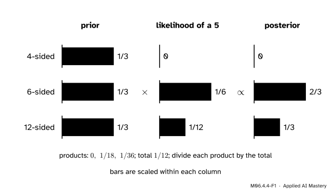
Each die is a hypothesis about where the 5 came from. Before the roll they are equally likely, \({1/3}\) each. Now ask how likely a 5 is under each one: impossible for the 4-sided die, \({1/6}\) for the 6-sided die and \({1/12}\) for the 12-sided die.
M06.4.4-F1
The Bayes table as a picture. Multiply each prior by its likelihood, then rescale so that the results add up to 1.
The 4-sided die is ruled out. The other two started level, and a 5 is twice as likely from the 6-sided die as from the 12-sided one, so after the roll the 6-sided die is twice as likely: \({2/3}\) against \({1/3}\). The posterior is the prior reshaped by the likelihood, then rescaled to add up to 1.
Build it up
Step 1. The hypotheses split the sample space. Exactly one die was taken out, so the three hypotheses are disjoint and together cover every possibility. They partition\(\Omega\), as the spam and not-spam emails did in M06.4.1, only now with three pieces.
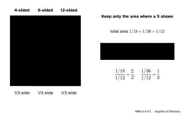
Step 2. Each prior is a strip. Draw \(\Omega\) as a unit square and cut it into three strips of width \({1/3}\), one for each die.
Step 3. Each likelihood is a height. Inside each strip, shade the part where the die shows a 5: height 0, \({1/6}\) and \({1/12}\). The shaded area in a strip is its width times its height, the prior times the likelihood: 0, \({1/18}\) and \({1/36}\).
M06.4.4-F2
Prior as width, likelihood as height, their product as area. The evidence is the total yellow area, and each posterior is its strip’s share of that area.
Step 4. The evidence is the total shaded area. By the law of total probability, \({\Prob(5) = 0 + 1/18 + 1/36 = 1/12}\).
Step 5. Zoom in. We know a 5 came up, so we are somewhere in the yellow area. The 6-sided die holds \({(1/18)/(1/12) = 2/3}\) of it, and the 12-sided die \({(1/36)/(1/12) = 1/3}\).
The formal statement
NoteBayes’ rule for many hypotheses
Let \({H_1, \dots, H_k}\) partition \(\Omega\), each with \({\Prob(H_i) > 0}\), and let \({\Prob(E) > 0}\). Then for each \(i\),
Derivation. Bayes’ rule from M06.4.1 holds for any one event \(H_i\): \({\Prob(H_i \mid E)} = {\Prob(E \mid H_i)\,\Prob(H_i) / \Prob(E)}\). Because the \(H_j\) partition \(\Omega\), the law of total probability (M06.3.3) gives
and the denominator only makes the column add up to 1. That gives a four-step recipe, one row per hypothesis:
write each prior;
write the likelihood of the evidence under each hypothesis;
multiply across, and add the products: the total is \({\Prob(E)}\);
divide each product by the total to get the posterior.
Picking the largest posterior is a classifier. To guess the hypothesis, pick the row with the largest posterior, the maximum a posteriori or MAP choice. The division does not change which row is largest, so the products alone decide.
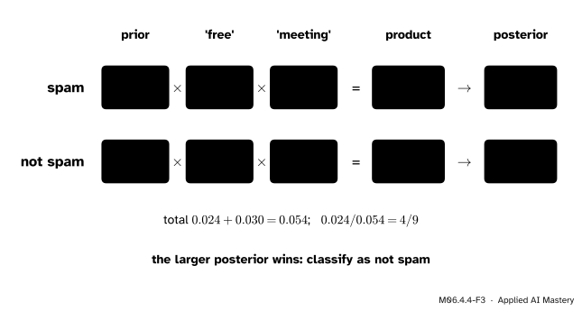
A first naive Bayes classifier. Add a second word to the inbox: ‘meeting’ is in 4 of the 40 spam emails and in 30 of the 60 others, so \({\Prob(\text{meeting} \mid \text{spam}) = 0.1}\) and \({\Prob(\text{meeting} \mid \text{not spam}) = 0.5}\). An email contains both words. To use Bayes’ rule we need the likelihood of both words under each class. Naive Bayes assumes that the words are conditionally independent given the class (M06.3.4), so the likelihood of both is the product of the likelihoods of each:
Naive Bayes is a Bayes table whose likelihood is a product, one factor per word. ‘free’ pushes towards spam, ‘meeting’ pushes harder the other way.
The total is 0.054, so \({\Prob(\text{spam} \mid \text{free, meeting})} = {0.024/0.054} = {4/9}\), about 0.44, and the classifier says “not spam”. In odds, this is the previous lesson: prior odds \({0.4/0.6}\), times a likelihood ratio of 6 for ‘free’, times \({0.1/0.5 = 1/5}\) for ‘meeting’, gives \({0.8}\), or 4 to 5. Taking logs turns the product into a sum, one term per word, which is why naive Bayes and logistic regression are close relatives (ML02.6). Hypotheses that form a continuous range, such as an unknown coin bias between 0 and 1, need a density in place of the table, and wait for S04.1.
Worked example
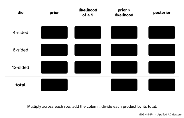
Which die rolled the 5? Fill in the table.
M06.4.4-F4
The worked table. The yellow total is the evidence \({\Prob(5) = 1/12}\).
Every prior is \({1/3}\), so each product is \({1/3}\) times the likelihood:
die
likelihood
product
posterior
4-sided
0
0
0
6-sided
\({1/6}\)
\({1/18}\)
\({2/3}\)
12-sided
\({1/12}\)
\({1/36}\)
\({1/3}\)
total
\({1/12}\)
1
The products add to \({2/36 + 1/36 = 3/36 = 1/12}\). Dividing, \({(1/18)/(1/12) = 12/18 = 2/3}\) and \({(1/36)/(1/12) = 12/36 = 1/3}\). The MAP guess is the 6-sided die, and it is wrong one time in three.
Notice what the evidence did to each row. The 4-sided die’s likelihood was 0, so its posterior is 0 no matter what its prior was. The other two rows kept their prior ratio of 1 to 1, multiplied by their likelihood ratio, \({(1/6)/(1/12) = 2}\): odds of 2 to 1, as in M06.4.3.
Code
First a Bayes table from scratch, with exact fractions. It takes a list of priors and a list of likelihoods and returns the posteriors.
from fractions import Fraction as Frdef bayes_table(priors, likelihoods):"""Posteriors for hypotheses that partition the sample space.""" products = [p * l for p, l inzip(priors, likelihoods)] total =sum(products) # the evidence, by total probabilityreturn [x / total for x in products], totaldice = ["4-sided", "6-sided", "12-sided"]priors = [Fr(1, 3)] *3likes_5 = [Fr(0), Fr(1, 6), Fr(1, 12)] # chance of a 5 on each dieposteriors, evidence = bayes_table(priors, likes_5)print("P(5) =", evidence, " posteriors:", [str(p) for p in posteriors])print("MAP guess:", dice[posteriors.index(max(posteriors))])
A simulation: pick a die at random, roll it, and keep only the rolls that show a 5.
import numpy as nprng = np.random.default_rng(seed=5)n =600_000sides = rng.choice([4, 6, 12], size=n)rolls = rng.integers(1, sides +1) # a fair roll of each chosen diefives = rolls ==5shares = [np.mean(sides[fives] == s) for s in (4, 6, 12)]print(f"{fives.sum()} rolls show a 5; shares by die:", np.round(shares, 3))
49964 rolls show a 5; shares by die: [0. 0.667 0.333]
Now naive Bayes for the inbox, from scratch with a NumPy array. Row 0 is spam and row 1 is not spam; column 0 is ‘free’ and column 1 is ‘meeting’. For an email with word indicators \(x\), each word contributes \({\Prob(\text{word} \mid \text{class})}\) when it is present and one minus that when it is absent.
prior = np.array([0.4, 0.6]) # spam, not spamp_word = np.array([[0.6, 0.1], # spam: P(free), P(meeting) [0.1, 0.5]]) # not spam: P(free), P(meeting)def naive_bayes(x):"""P(spam), P(not spam) for an email with word indicators x = (free, meeting).""" likelihood = np.prod(np.where(np.array(x) ==1, p_word, 1- p_word), axis=1) products = prior * likelihoodreturn products / products.sum()for x in [(1, 1), (1, 0), (0, 0), (0, 1)]: post = naive_bayes(x) label ="spam"if post[0] > post[1] else"not spam"print(f"free={x[0]} meeting={x[1]}: P(spam) = {post[0]:.3f} -> {label}")
scikit-learn’s BernoulliNB learns the same table from the 100 labelled emails. Setting alpha=0 with force_alpha=True turns off its smoothing, so it uses the raw counts, as we did.
Naive Bayes only uses the counts of each word within each class. Which spam emails hold both words does not enter it, which is exactly what “naive” means.
Explore
The frequency grid of lesson M06.4.2 is a Bayes table with two rows, drawn as people. The blue cells are the first row and the sky-blue cells the second; gathering the positives is adding the product column.
Pitfalls
M06.4.4-F5
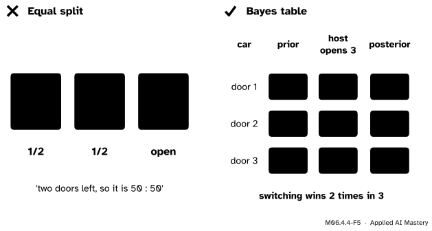
Wrong beside right. The host’s choice is evidence, and its likelihood depends on where the car is.
“Two doors are left, so each has a probability of 1/2.”
In the Monty Hall game a car is behind one of three doors, you pick door 1, and the host, who knows where the car is and always opens a door with a goat, opens door 3. The hypotheses are the three places for the car, each with prior \({1/3}\). The evidence is “the host opens door 3”. If the car is behind door 1 he could open door 2 or 3, and picks door 3 with probability \({1/2}\). If it is behind door 2 he must open door 3: probability 1. If it is behind door 3 he cannot open it: probability 0. The products are \({1/6}\), \({1/3}\) and 0, with total \({1/2}\), so the posteriors are \({1/3}\), \({2/3}\) and 0. Switching wins two times in three.
“The product column is the posterior.”
The products, 0, \({1/18}\) and \({1/36}\), add up to \({1/12}\), not 1. They rank the hypotheses correctly, so the MAP choice can be read from them, but to state how sure you are you must divide by the total.
“Naive Bayes gives the true probability that an email is spam.”
Only if the words really are conditionally independent given the class. Words that travel together, such as ‘free’ and ‘offer’, each multiply in the same evidence, so the products overstate it and the posteriors come out too close to 0 or 1, even when the class they pick is right. The same thing happened with the repeated test in M06.4.3.
Check yourself
Recall
1. State Bayes’ rule for hypotheses \({H_1, \dots, H_k}\) that partition \(\Omega\).
Show answer
Each posterior \({\Prob(H_i \mid E)}\) is the product \({\Prob(E \mid H_i)\,\Prob(H_i)}\) divided by the sum of these products over all the hypotheses, which is the evidence \({\Prob(E)}\).
2. What are the four steps of a Bayes table?
Show answer
Write the priors, write the likelihoods, multiply across and add the products (the total is the evidence), then divide each product by the total.
3. Why is the posterior of the 4-sided die 0 after a 5?
Show answer
Its likelihood is 0, because a 4-sided die cannot show a 5. A product with a factor of 0 is 0, whatever the prior.
4. What does “the posterior is proportional to prior times likelihood” mean?
Show answer
Every row is divided by the same number, the evidence, so the posteriors are the products scaled to add up to 1. Their ratios are the ratios of the products.
5. What does naive Bayes assume about the words of an email?
Show answer
That they are conditionally independent given the class, so that the likelihood of several words is the product of the likelihoods of each word.
Exercises
1.★ Start again with the three dice, each with prior \({1/3}\). The roll shows a 3. Find the three posteriors.
Show solution
The likelihoods are \({1/4}\), \({1/6}\) and \({1/12}\), so the products are \({1/12}\), \({1/18}\) and \({1/36}\), that is \({3/36}\), \({2/36}\) and \({1/36}\). They add to \({6/36 = 1/6}\), and the posteriors are \({1/2}\), \({1/3}\) and \({1/6}\). Every die can show a 3, and the die with the fewest faces shows it most often.
2.★★ After the 5, the same die is rolled again and shows a 3. Update the table, using the posteriors after the 5 as the new priors. Then check by treating “a 5, then a 3” as one piece of evidence from the original priors.
Show solution
New priors 0, \({2/3}\), \({1/3}\); likelihoods of a 3 are \({1/4}\), \({1/6}\), \({1/12}\). The products are 0, \({1/9}\) and \({1/36}\), that is 0, \({4/36}\) and \({1/36}\), with total \({5/36}\). The posteriors are 0, \({4/5}\) and \({1/5}\). In one step: rolls of the same die are conditionally independent given the die, so the likelihoods of “5 then 3” are 0, \({1/36}\) and \({1/144}\). Times \({1/3}\) they are 0, \({1/108}\) and \({1/432}\), that is 0, \({4/432}\) and \({1/432}\), with total \({5/432}\): again 0, \({4/5}\) and \({1/5}\).
3.★★★ With the naive Bayes classifier of this lesson, find \({\Prob(\text{spam} \mid \text{free, no meeting})}\) twice: with the Bayes table, and as a sum of log-odds.
Show solution
Table: the likelihood of “no meeting” is \({1 - 0.1 = 0.9}\) for spam and \({1 - 0.5 = 0.5}\) for the others. The products are \({0.4 \times 0.6 \times 0.9 = 0.216}\) and \({0.6 \times 0.1 \times 0.5 = 0.03}\), with total 0.246, so the posterior is \({0.216/0.246 = 36/41 \approx 0.878}\). Log-odds: start from the prior, \({\ln(0.4/0.6)}\), and add one likelihood ratio per word:
So the odds are 7.2 and the probability is \({7.2/8.2 = 36/41}\), the same.
Summary card
Prior times likelihood in every row, then divide by the total.
M06.4.4-F1
A 5: posteriors 0, 2/3, 1/3.
Many hypotheses.\({\Prob(H_i \mid E) \propto \Prob(E \mid H_i)\,\Prob(H_i)}\), scaled to add up to 1.
The scale. The products add up to the evidence \({\Prob(E)}\).
Classify. Pick the largest posterior; the products alone decide.
Naive Bayes. Likelihood of several words = product of one likelihood per word.
Sources and next steps
Sources. Each was opened and checked against this lesson on 12 November 2026.
Charles M. Grinstead and J. Laurie Snell, Introduction to Probability, second edition, Section 4.1. Bayes’ formula for hypotheses \({H_1, \dots, H_m}\) that partition \(\Omega\), derived from equations (4.1) to (4.3), and Example 4.6, the Monty Hall problem, where the car is behind door 2 with conditional probability \({2/3}\).
Jeremy Orloff and Jonathan Bloom, Reading 11: Bayesian updating with discrete priors, MIT OpenCourseWare 18.05, Spring 2022. Section 3 sets out the Bayesian update table (hypothesis, prior, likelihood, Bayes numerator, posterior) and states that the posterior is proportional to likelihood times prior; Section 4 updates again with the posterior as the new prior.
Jeremy Orloff and Jonathan Bloom, Reading 12b: Bayesian updating, odds, Section 4.1: a die drawn from five with 4, 6, 8, 12 and 20 sides, whose rolls are conditionally independent given the die but not independent.
scikit-learn, Naive Bayes, User Guide Section 1.9: the naive conditional independence assumption and the rule of picking the class with the largest prior times product of likelihoods; Section 1.9.4 gives the Bernoulli rule used here. The BernoulliNB page documents alpha and force_alpha.
Next.M06.5, Discrete random variables, gives a number to every outcome. Later, ML02.6 builds naive Bayes in full, and S04.1 replaces the table with a prior over a continuous parameter.