When every outcome is equally likely, a probability is a count: the outcomes in the event over all the outcomes. Derive that rule from the axioms, count sample spaces in stages with the multiplication rule, and see why the 11 sums of two dice are not equally likely.
Derive P(A) = |A| / |Omega| from the three axioms when all outcomes of a finite sample space are equally likely.
Count a sample space in stages with the multiplication rule, drawn as a tree.
Compute probabilities on the two-dice grid and for a random PIN by counting cells or paths.
Spot a list of outcomes that are not equally likely, and repair it by listing finer outcomes with itertools.product.
In review. The maths and code on this page are checked by automated tests on every change, but an independent reader has not signed it off yet. Spot a mistake or a confusing step? Tell us.
The question
Roll two fair dice and add them. There are 11 possible sums, from 2 to 12. Is each sum’s chance therefore 1/11? And a thief who tries one random 4-digit PIN: how small is the chance that it opens your phone?
Intuition
Some experiments have a built-in symmetry. A fair die has six faces and nothing to tell them apart, so no face can be favoured over another. When every outcome has the same chance, finding a probability needs no new idea at all. You count.
M06.2.1-F1
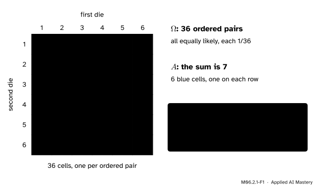
Two fair dice give 36 ordered pairs, all equally likely. The event “the sum is 7” covers 6 of the cells, so its probability is 6/36 = 1/6.
The picture is the whole lesson. The sample space \(\Omega\) of two dice is a 6 by 6 grid: the first die picks the column, the second picks the row. The 36 cells are equally likely. The event “the sum is 7” is a set of cells, and its probability is the share of the grid it covers.
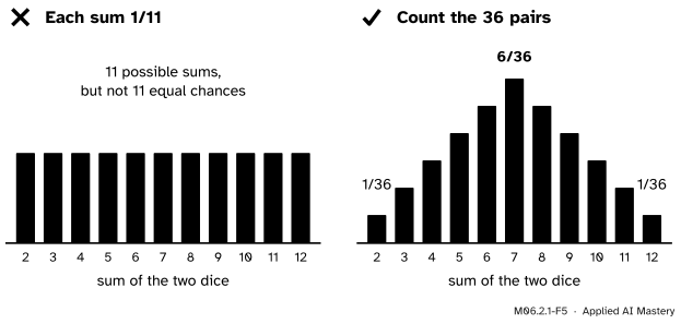
The rule has a hidden condition, and most mistakes in this lesson come from forgetting it: the outcomes you count must really be equally likely. The sum itself has 11 values, but the values are not equally likely, because 7 can be made in six ways and 2 in only one.
Build it up
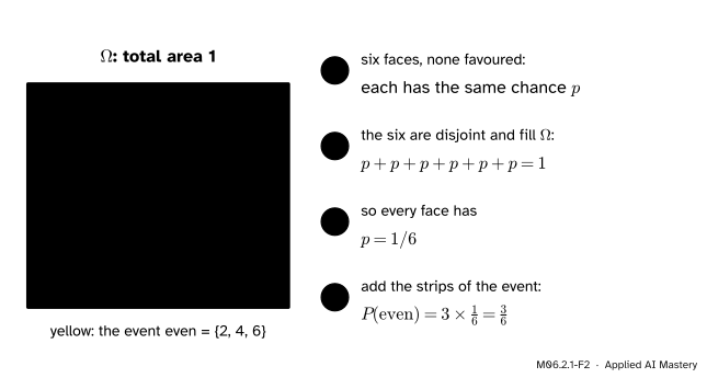
Step 1. The axioms fix the size of equal chances. Take a fair die. Call the chance of each face \(p\); symmetry says it is the same \(p\) for all six. The faces are disjoint and together they make up \(\Omega\), so the second and third axioms of lesson M06.1.3 give \(6p = 1\), and so \(p = 1/6\).
M06.2.1-F2
The area picture of the axioms. Six equal strips must share a total area of 1, so each has area 1/6, and an event’s area is its number of strips times 1/6.
Step 2. An event is a handful of strips. The event “even” is the three strips 2, 4 and 6. Additivity adds their areas: \({3 \times 1/6 = 3/6}\). In general an event that holds \(m\) of the six faces has probability \(m/6\).
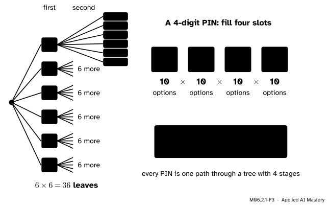
Step 3. Count big spaces in stages. Listing 6 outcomes is easy; listing 10,000 PINs is not. The multiplication rule of lesson M01.8.1 counts them without a list: if an outcome is built in stages, and stage 1 has \(n_1\) options, then stage 2 has \(n_2\) options whatever happened at stage 1, and so on, the number of outcomes is the product \({n_1 n_2 \cdots n_k}\).
M06.2.1-F3
Stages multiply. Each first-die branch carries 6 second-die leaves, so two dice have \({6 \times 6 = 36}\) outcomes; four digits with 10 options each make 10,000 PINs.
A tree draws the rule: one level per stage, one branch per option, and every outcome is a path from the root to a leaf. The number of leaves is the product of the branch counts.
The formal statement
NoteEqually likely outcomes
Let \(\Omega\) be a finite sample space with \(N = |\Omega|\) outcomes, and suppose every outcome has the same probability. Then each outcome has probability \(1/N\), and every event \(A\) has
\[
\Prob(A) = \frac{|A|}{|\Omega|}.
\]
Proof. Write \(\Omega = \{\omega_1, \dots, \omega_N\}\) and let \(p\) be the common probability of each one-outcome event \(\{\omega_i\}\). These \(N\) events are disjoint and their union is \(\Omega\), so the axioms give
\[
\begin{aligned}
1 &= \Prob(\Omega) \\
&= \Prob(\{\omega_1\}) + \cdots + \Prob(\{\omega_N\}) \\
&= N p .
\end{aligned}
\]
So \(p = 1/N\). An event \(A\) is the disjoint union of its own \(|A|\) outcomes, so additivity again gives
That is the whole proof, and it shows what the rule needs: a finite \(\Omega\), and equal chances. This assignment of probabilities is called the uniform distribution on \(\Omega\).
NoteThe multiplication rule for counting
If an outcome is made in \(k\) stages, with \(n_i\) options at stage \(i\) whatever the earlier stages gave, then the number of outcomes is \({n_1 \times n_2 \times \cdots \times n_k}\).
Two consequences follow at once. Two dice: \({6 \times 6 = 36}\). A 4-digit PIN, digits 0 to 9 and repeats allowed: \({10^4 = 10{,}000}\).
Worked example
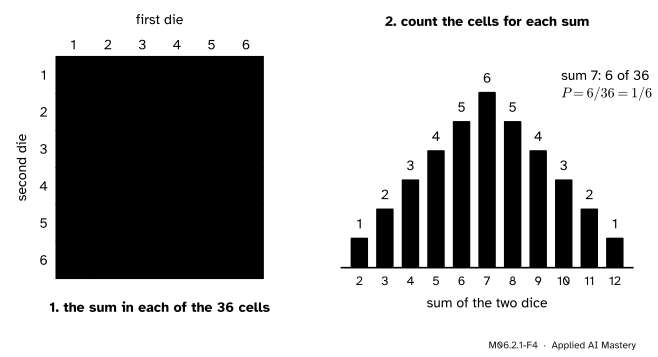
Two dice. Write the sum in each of the 36 cells, then count the cells that hold each sum.
M06.2.1-F4
The trace of the worked example. Equal sums lie on the diagonals from top right to bottom left, so the counts climb from 1 to 6 and fall back to 1.
The counts for the sums 2 to 12 are 1, 2, 3, 4, 5, 6, 5, 4, 3, 2, 1, which add up to 36 as they must. So
At least one six. The cells with a six fill the last column (6 cells) and the last row (6 cells), but the corner (6, 6) is in both, so \({6 + 6 - 1 = 11}\) cells. The probability is 11/36. The complement rule of lesson M06.1.4 gives the same: the cells with no six form a 5 by 5 block of 25, and \({1 - 25/36 = 11/36}\).
The PIN. All 10,000 PINs are equally likely if the PIN was chosen at random, so one guess succeeds with probability \({1/10{,}000 = 0.0001}\). Three different guesses cover 3 outcomes: \({3/10{,}000}\). The event “the PIN starts with 0” fixes the first stage and leaves \({10 \times 10 \times 10 = 1{,}000}\) PINs, so its probability is \({1{,}000/10{,}000 = 1/10}\).
Code
First from scratch. itertools.product builds the ordered pairs, and Fraction keeps every probability exact, so the answers print as 1/6 rather than 0.16666.
from fractions import Fractionfrom itertools import productomega =list(product(range(1, 7), repeat=2)) # 36 ordered pairs (first, second)def prob(event, omega):"""P(A) = |A| / |Omega|, for equally likely outcomes. `event` is a test on one outcome."""return Fraction(sum(1for w in omega if event(w)), len(omega))p7 = prob(lambda w: w[0] + w[1] ==7, omega)p2 = prob(lambda w: w[0] + w[1] ==2, omega)p_six = prob(lambda w: 6in w, omega)print(len(omega), p7, p2, p_six)pins =list(product(range(10), repeat=4))p_zero = prob(lambda pin: pin[0] ==0, pins)print(len(pins), p_zero)
36 1/6 1/36 11/36
10000 1/10
Now let NumPy roll the dice 100,000 times. The share of sevens should sit close to 1/6, about 0.1667, though not exactly on it.
import numpy as nprng = np.random.default_rng(2026)rolls = rng.integers(1, 7, size=(100_000, 2)) # each row: first die, second dieshare7 = np.mean(rolls.sum(axis=1) ==7)print(round(float(share7), 4))
0.166
The simulation agrees with the count to within a few thousandths. The count is exact; the simulation is evidence that the model of two fair, separate dice is the right one.
Explore
This module’s interactive, the counting explorer, lives in lesson M06.2.3. There you draw from a bag of numbered balls, switch order and replacement on and off, and see which outcomes group together and which groups are equally likely.
Pitfalls
M06.2.1-F5
Wrong beside right. Listing the 11 sums and giving each 1/11 ignores how many pairs make each sum. Counting the 36 equally likely pairs gives the triangle.
“There are 11 sums, so each has probability 1/11.”
The formula \(|A|/|\Omega|\) is only valid when the outcomes in \(\Omega\) are equally likely, and the 11 sums are not. Choose outcomes fine enough to be equally likely (the 36 ordered pairs), count there, and only then group them by sum.
M06.2.1-F6
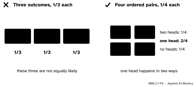
The same mistake with two coins. “One head” happens in two ways, HT and TH, so it has twice the chance of “two heads”.
“Two coins can show no heads, one head or two heads, so each has probability 1/3.”
Again the three outcomes are not equally likely. The four ordered pairs HH, HT, TH, TT are, and they give 1/4, 2/4 and 1/4. Grinstead and Snell discuss this example: describing two pennies by the number of heads is a correct description of what can happen, but the uniform distribution on it does not match experience.
“Every experiment has equally likely outcomes if I list them carefully enough.”
Not so. A loaded die (lesson M06.1.3) has six outcomes with different chances, and no finer list makes them equal. Equal chances are a modelling assumption, justified by symmetry or by experiment. In machine learning the same assumption hides in “shuffle the data and take a random batch”: the shuffle is designed so that every order is equally likely.
Check yourself
Recall
1. State the rule for \(\Prob(A)\) when all outcomes are equally likely, and its two conditions.
Show answer
\(\Prob(A) = |A|/|\Omega|\). The sample space must be finite, and every outcome must have the same probability.
2. How many outcomes do two dice have, and why?
Show answer
The first die has 6 options and, for each of them, the second has 6, so the multiplication rule gives \({6 \times 6 = 36}\) ordered pairs.
3. What is the probability that the sum of two dice is 7?
Show answer
6 of the 36 pairs give 7: (1, 6), (2, 5), (3, 4), (4, 3), (5, 2), (6, 1). So 6/36 = 1/6.
4. Why is the chance of each sum of two dice not 1/11?
Show answer
The 11 sums are not equally likely: a sum of 7 comes from 6 pairs and a sum of 2 from 1. The rule \(|A|/|\Omega|\) needs equally likely outcomes, which the 36 pairs are and the 11 sums are not.
5. How many 4-digit PINs are there, and what is the chance that one random guess is right?
Show answer
\({10^4 = 10{,}000}\) PINs, so one guess is right with probability 1/10,000 if the PIN was chosen at random.
Exercises
1.★ Two fair dice are rolled. Find the probability that the two dice show the same number (a double), and the probability that the sum is at most 4.
Show solution
Doubles are the 6 cells (1, 1) to (6, 6) on the main diagonal: 6/36 = 1/6. A sum of at most 4 is a sum of 2, 3 or 4, which have 1, 2 and 3 cells: \({(1 + 2 + 3)/36 = 6/36 = 1/6}\).
2.★★ A password has 3 lower-case letters (26 options each) followed by 2 digits. How many passwords are there? If one is chosen at random, what is the chance that it ends in 00, and the chance that its first letter is a vowel (a, e, i, o, u)?
Show solution
By the multiplication rule there are \({26^3 \times 10^2}\) passwords, which is \({17{,}576 \times 100}\), or 1,757,600. Ending in 00 fixes the last two stages and leaves \({26^3 = 17{,}576}\) passwords, so the probability is 17,576/1,757,600, which is 1/100. A vowel first leaves \({5 \times 26^2 \times 10^2}\) passwords, which is 338,000, so the probability is 338,000/1,757,600, which is 5/26. In both cases the other stages cancel, which is a quick check.
3.★★★ Three fair coins are tossed. A friend argues: “the number of heads is 0, 1, 2 or 3, so P(exactly one head) = 1/4.” Find the right answer by listing equally likely outcomes, and explain where the argument fails.
Show solution
The equally likely outcomes are the \({2^3 = 8}\) ordered triples HHH, HHT, HTH, HTT, THH, THT, TTH, TTT. Exactly one head: HTT, THT and TTH, so the probability is 3/8. The friend’s four head counts are not equally likely: 0 and 3 heads each come from 1 triple, and 1 and 2 heads each from 3. The rule \(|A|/|\Omega|\) may only be used on the 8 triples.
Summary card
Equally likely outcomes turn probability into counting.
M06.2.1-F1
Count the cells, divide by 36.
The rule. If all \(N\) outcomes are equally likely, \(\Prob(A) = |A|/|\Omega|\).
Where it comes from. The axioms force each outcome to have probability \(1/N\).
Counting \(\Omega\). Stages multiply: two dice 36, a 4-digit PIN 10,000.
The trap. Count only outcomes that really are equally likely; group them afterwards.
Sources and next steps
Sources. Each was opened and checked against this lesson on 12 November 2026.
Charles M. Grinstead and J. Laurie Snell, Introduction to Probability, second edition (free under the GNU Free Documentation License). Definition 1.3 defines the uniform distribution on a finite sample space, each outcome having probability one over the number of outcomes; Example 3.14 discusses two pennies described by the number of heads against the four ordered pairs.
Hossein Pishro-Nik, Introduction to Probability, Statistics, and Random Processes, Section 2.1, Counting: for a finite sample space with equally likely outcomes, \(\Prob(A) = |A|/|S|\), so finding a probability becomes a counting problem; the multiplication principle is used to count passwords.
Python Software Foundation, itertools.product and fractions.Fraction, Python 3.12 documentation: the Cartesian product with repeat, and exact rational numbers.