Standardise the mean of n independent draws and its distribution settles onto the same bell, whatever the draws looked like. See it on dice, a skewed delay, two humps and a coin, learn why only μ and σ survive, and meet a case where the bell never comes.
Standardise a sample mean, Zₙ = (X̄ₙ − μ)/(σ/√n), and show that the sum gives the same Zₙ.
State the central limit theorem as P(Zₙ ≤ z) → Φ(z), with its conditions: independent, identically distributed, finite variance.
Compare exact distributions of sums with the normal curve, and explain in words why only μ and σ survive the averaging.
Recognise a case where the theorem does not apply: draws with no finite variance, such as the Cauchy distribution.
In review. The maths and code on this page are checked by automated tests on every change, but an independent reader has not signed it off yet. Spot a mistake or a confusing step? Tell us.
The question
Heights, measurement errors, exam marks and the noise in a mini-batch gradient all come out roughly bell-shaped, even though nothing about a single gene, a single nudge of a ruler or a single training example is bell-shaped. Why does one curve turn up in so many places, and when can we rely on it?
From the last lesson
1. State Chebyshev’s inequality with \(k\) standard deviations.
For i.i.d. draws with mean \(\mu\) and finite variance, \({\Prob(\abs{\bar{X}_n - \mu} \ge \varepsilon)}\)\({\to 0}\) as \(n\) grows, for every \({\varepsilon > 0}\).
Intuition
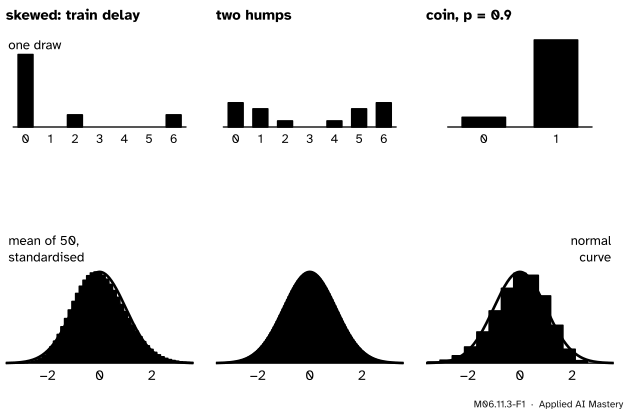
The law of large numbers says the average closes in on \(\mu\). If we zoom in on it at the right scale, so that it stops shrinking, we can watch its shape. The picture does that for three sources that look nothing alike.
M06.11.3-F1
Top: three sources, one skewed, one with two humps, one a lopsided coin. Bottom: the exact distribution of the mean of 50 draws from each, standardised. All three sit on the same normal curve.
The skew, the two humps and the lopsided coin have all washed out. What is left is the bell of M06.6.4. That is the central limit theorem, one of the most useful facts in all of probability.
Build it up
Step 1. Zoom to a fixed scale. The mean has centre \(\mu\) and spread \({\sigma/\sqrt{n}}\), so subtract the centre and divide by the spread:
Like any standardised variable (M06.7.4), \({\E[Z_n] = 0}\) and \({\operatorname{Var}(Z_n) = 1}\) for every \(n\). Multiply top and bottom by \(n\) and the same variable is written with the sum \({S_n = n\bar{X}_n}\):
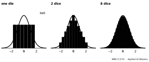
Step 2. Watch dice. One die is flat. The sum of two is a triangle. The sum of eight is already hard to tell from the bell.
M06.11.3-F2
The standardised sum of 1, 2 and 8 dice, worked out exactly by convolution, against the standard normal density. Bar areas are probabilities.
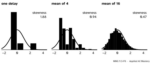
Step 3. Watch a skew fade. The train delay is very lopsided: skewness \({15/8 \approx 1.88}\) (M06.7.4). Averaging is slower to iron that out, but it does.
M06.11.3-F6
The standardised mean of 1, 4 and 16 train delays. The skewness halves each time \(n\) is multiplied by 4: 1.88, 0.94, 0.47.
Step 4. The Galton board. A ball’s bin is its number of right bounces, a sum of \(n\) Bernoulli variables (M06.5.1), so the bins of a board with \(n\) rows follow \({\mathrm{Bin}(n, p)}\). With many rows the pile of balls takes the bell shape, tilted board or not: the theorem for coin flips. Try it on the Galton board of M06.5.2: set 10 rows and the chance of bouncing right to \({p = 0.3}\), and drop a few hundred balls.
The formal statement
NoteTheorem: the central limit theorem
Let \(X_1, X_2, \dots\) be i.i.d. with mean \(\mu\) and finite variance \({\sigma^2 > 0}\), and let \({Z_n}\)\({= (\bar{X}_n - \mu)/(\sigma/\sqrt{n})}\). Then for every number \(z\),
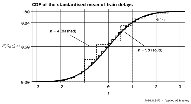
The theorem is about CDFs, so a discrete variable is allowed: its staircase CDF hugs the smooth \(\Phi\) more and more closely.
M06.11.3-F3
The CDF of the standardised mean of train delays at \({n = 4}\) (dashed) and \({n = 50}\) (solid). The largest gap to \(\Phi\) shrinks from 0.22 to 0.046.
We do not prove the theorem here; the proof needs the transforms of M07.2 and comes in M07.5. Note what it asks for: independence, one common distribution, and a finite variance. Nothing about the shape.
Why only \(\mu\) and \(\sigma\) survive. Standardising fixes the centre at 0 and the spread at 1 for every \(n\), so \(\mu\) and \(\sigma\) are used up by construction. Every other feature of a single draw, its skew, its humps, the gaps between its values, is shared among \(n\) terms. Each term’s quirks push in independent directions and mostly cancel, and what does not cancel is shrunk: the skewness of the mean is the skewness of one draw divided by \(\sqrt{n}\). In the limit nothing but the bell is left.
Go deeper: the skewness of a mean falls like 1 over root n
Write \({D_i = X_i - \mu}\), so \({\E[D_i] = 0}\), \({\E[D_i^2] = \sigma^2}\) and \({\E[D_i^3] = m_3}\). Expand \({(D_1 + \dots + D_n)^3}\). A term \({D_i^2 D_j}\) with \({i \ne j}\) has expectation \({\E[D_i^2]\,\E[D_j] = 0}\) by independence, and so does every term \({D_i D_j D_k}\) with three different indices. Only the \(n\) cubes remain, so the third central moment of \(S_n\) is \({n m_3}\). Its variance is \({n\sigma^2}\), so its skewness is
where \(\gamma\) is the skewness of one draw. The mean \({S_n/n}\) has the same skewness, because skewness ignores shifts and positive stretches. For the delay: \({1.875/\sqrt{4} \approx 0.94}\).
Worked example
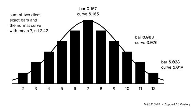
How close is the bell for two dice? The sum \({S_2}\) has \({\mu = 7}\) and \({\sigma = \sqrt{35/6} \approx 2.415}\). A bar of width 1 at \(k\) has area \({\Prob(S_2 = k)}\); the normal curve with the same mean and spread has height
there, which is about the area under the curve across that bar.
M06.11.3-F4
The sum of two dice against the normal curve with the same mean and spread. Already close in the middle; further off in the tails.
At \({k = 7}\): \({z = 0}\), and \({\varphi(0)}\)\({= 1/\sqrt{2\pi}}\)\({\approx 0.3989}\), so the curve gives \({0.3989/2.415 \approx 0.165}\) against the exact \({6/36 \approx 0.167}\).
At \({k = 10}\): \({z = 3/2.415 \approx 1.242}\) and \({\varphi(1.242) \approx 0.184}\), so the curve gives \({0.184/2.415 \approx 0.076}\) against \({3/36 \approx 0.083}\).
At \({k = 12}\): \({z \approx 2.070}\), \({\varphi(2.070) \approx 0.047}\), so the curve gives about 0.019 against \({1/36 \approx 0.028}\).
The middle is right within 1%; the edge is off by a third. With six dice the match is closer: the exact \({\Prob(S_6 = 21)}\)\({= 4332/46656}\)\({\approx 0.0928}\) against \({\varphi(0)/\sqrt{17.5}}\)\({\approx 0.0954}\).
Code
From scratch: exact distributions by convolution, and the largest gap between the staircase CDF of \({Z_n}\) and \(\Phi\), written with math.erf as in M06.6.4.
import mathimport numpy as npdef Phi(z):return0.5* (1+ math.erf(z / math.sqrt(2)))def cdf_gap(pmf, n):"""Largest |P(Z_n <= z) - Phi(z)| for the standardised sum of n draws from pmf on 0, 1, 2, ...""" x = np.arange(len(pmf)) mu, var = (x * pmf).sum(), ((x - (x * pmf).sum()) **2* pmf).sum() probs = np.array([1.0])for _ inrange(n): probs = np.convolve(probs, pmf) z = (np.arange(len(probs)) - n * mu) / math.sqrt(n * var) after = np.cumsum(probs) # the staircase just after each jump before = after - probs # and just before it target = np.array([Phi(v) for v in z])returnmax(np.abs(after - target).max(), np.abs(before - target).max())delay = np.array([6, 0, 1, 0, 0, 0, 1]) /8# 0, 2 or 6 minutesdie = np.array([0, 1, 1, 1, 1, 1, 1]) /6for n in (1, 4, 16, 50):print(f"train delay, n = {n:2}: largest CDF gap {cdf_gap(delay, n):.3f}")print("one die:", round(cdf_gap(die, 1), 3), " eight dice:", round(cdf_gap(die, 8), 3))
train delay, n =  1: largest CDF gap 0.441
train delay, n =  4: largest CDF gap 0.219
train delay, n = 16: largest CDF gap 0.084
train delay, n = 50: largest CDF gap 0.046
one die: 0.143   eight dice: 0.042
Now simulation: means of 50 draws from each source, standardised. If the theorem is at work, about 68.3% of them lie within 1 and 95.4% within 2, as for a normal variable.
from scipy import statsrng = np.random.default_rng(3)sources = {"train delay": ([0, 2, 6], [0.75, 0.125, 0.125]),"two humps": (range(7), np.array([4, 3, 1, 0, 1, 3, 4]) /16),"coin, p = 0.9": ([0, 1], [0.1, 0.9])}for name, (values, probs) in sources.items(): values, probs = np.asarray(values, dtype=float), np.asarray(probs) mu = (values * probs).sum() sigma = math.sqrt(((values - mu) **2* probs).sum()) means = rng.choice(values, p=probs, size=(20_000, 50)).mean(axis=1) z = (means - mu) / (sigma / math.sqrt(50))print(f"{name:14} within 1: {np.mean(abs(z) <=1):.3f} within 2: {np.mean(abs(z) <=2):.3f}"f" skewness of the means: {stats.skew(means):+.2f}")print("normal: within 1:", round(stats.norm.cdf(1) - stats.norm.cdf(-1), 3)," within 2:", round(stats.norm.cdf(2) - stats.norm.cdf(-2), 3))
train delay    within 1: 0.705  within 2: 0.962  skewness of the means: +0.26
two humps      within 1: 0.689  within 2: 0.955  skewness of the means: +0.03
coin, p = 0.9  within 1: 0.765  within 2: 0.971  skewness of the means: -0.35
normal:         within 1: 0.683  within 2: 0.954
The shares are close to the normal ones. The coin’s are the furthest off: its means take only 51 values, so whole bars sit on the edges \({\pm 1}\) and \({\pm 2}\). The skewness of the delay’s means is near \({1.875/\sqrt{50} \approx 0.27}\), as the deeper note predicts; simulated digits will differ a little on another machine.
Explore
M06.11-X1
Sample-mean machine
Pick a source and a sample size \(n\), then draw: each press takes \(n\) values and drops their mean into the histogram. Compare its centre and spread with \(\mu\) and \({\sigma/\sqrt{n}}\) in the read-out, and switch on the normal curve.
Things to try. Choose two humps and \({n = 1}\): the histogram copies the humps. Move to \({n = 2}\), then 5, then 20, drawing a few hundred means each time. Then take the coin and push \(p\) to 0.05 with \({n = 10}\): the expected number of heads is only 0.5, the means pile up at 0, and the bell fits badly. Raise \(n\) to 50 and it improves, though with only 2.5 heads expected per sample the read-out still warns.
Pitfalls
M06.11.3-F5
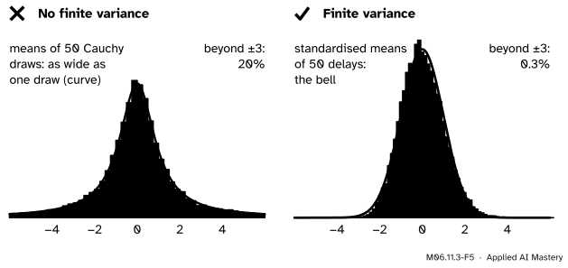
Wrong beside right. Averages of Cauchy draws, which have no finite variance, never become a bell: the mean of 50 is spread exactly like one draw. Averages of train delays do.
“Average enough of anything and you get a bell.”
The theorem needs a finite variance. The Cauchy distribution, with density \({1/(\pi(1 + x^2))}\), has tails so heavy that it has no mean and no variance, and the average of \(n\) Cauchy draws has exactly the same distribution as one draw. A fifth of the means of 50 still land more than 3 from the centre. Losses or gradients with very heavy tails, from outliers, can behave like this, which is one reason for clipping them.
“The theorem says the data become normal.”
The data keep their own distribution, skewed or two-humped. It is the distribution of the average (or the sum) that becomes normal. Testing whether a dataset “looks normal” says nothing about whether its mean is approximately normal.
“n = 30 is always enough.”
How large \(n\) must be depends on the source. For a symmetric one, such as dice, a handful of draws will do. For a coin with \({p = 0.01}\) and \({n = 30}\), the chance of no heads at all is \({0.99^{30} \approx 0.74}\), and no bell describes that. Skew shrinks only like \({1/\sqrt{n}}\).
Check yourself
Recall
1. Write the standardised mean \(Z_n\) in two ways.
For i.i.d. draws with mean \(\mu\) and finite variance \({\sigma^2 > 0}\), \({\Prob(Z_n \le z) \to \Phi(z)}\) for every \(z\).
3. What does the theorem need, and what does it not need?
Show answer
Independence, a common distribution and a finite variance. It does not need the draws to have any particular shape, or even to be continuous.
4. How does the skewness of the mean of \(n\) draws depend on \(n\)?
Show answer
It is the skewness of one draw divided by \(\sqrt{n}\).
5. Name a distribution whose averages never approach a bell, and say why.
Show answer
The Cauchy distribution: it has no finite variance (not even a mean), and the average of \(n\) draws has the same distribution as one draw.
Exercises
1.★ The mean of 25 draws has \({\mu = 10}\) and \({\sigma = 5}\) for one draw. Find \({Z_{25}}\) when the mean is 11, and use \(\Phi\) to estimate \({\Prob(\bar{X}_{25} \le 11)}\).
Show solution
\({\sigma/\sqrt{25} = 1}\), so \({Z_{25} = (11 - 10)/1 = 1}\), and \({\Prob(\bar{X}_{25} \le 11)}\)\({\approx \Phi(1)}\)\({\approx 0.841}\).
2.★★ The train delay has skewness \({15/8}\). How many delays must be averaged for the skewness of the mean to fall below 0.1?
Show solution
We need \({1.875/\sqrt{n} < 0.1}\), so \({\sqrt{n} > 18.75}\) and \({n > 351.6}\): at least 352 delays.
3.★★★ Use the normal curve to approximate \({\Prob(S_2 = 4)}\) for the sum of two dice, as in the worked example, and compare with the exact value. Why is the error the same as at \({k = 10}\)?
Show solution
\({z = (4 - 7)/2.415 \approx -1.242}\), and \({\varphi(-1.242)}\)\({= \varphi(1.242)}\)\({\approx 0.184}\), so the curve gives \({0.184/2.415 \approx 0.076}\). The exact value is \({3/36 \approx 0.083}\). Both the PMF of \(S_2\) and the normal curve are symmetric about 7, and 4 and 10 are both 3 away from 7, so both the bar and the curve height are the same at the two points.
Summary card
Standardised averages of i.i.d. draws with finite variance settle onto the bell.
\({\Prob(Z_n \le z) \to \Phi(z)}\); so \({\bar{X}_n \approx N(\mu, \sigma^2/n)}\).
Skewness of the mean: \({\gamma/\sqrt{n}}\).
Needs a finite variance: Cauchy averages never become normal.
Sources and next steps
Sources. Each was opened and checked against this lesson on 12 November 2026.
Jeremy Orloff and Jonathan Bloom, Reading 6b: Central Limit Theorem and the Law of Large Numbers, MIT OpenCourseWare 18.05, Spring 2022. Section 5.1 (standardisation), Section 5.2 (the two equal forms of \({Z_n}\), the approximations for \({\bar{X}_n}\) and \({S_n}\), and the precise statement \({F_{Z_n}(z) \to \Phi(z)}\)) and Section 5.6 (how big \(n\) must be).
Hossein Pishro-Nik, Central Limit Theorem, Section 7.1.2 of Introduction to Probability, Statistics, and Random Processes: the theorem for i.i.d. variables with \({0 < \sigma^2 < \infty}\) as convergence of the CDF of \({Z_n}\) to \(\Phi\).
Charles M. Grinstead and J. Laurie Snell, Introduction to Probability, second edition: Theorem 9.2 (the theorem for Bernoulli trials), Theorem 9.3 (the local approximation \({\varphi(x_j)/\sqrt{n\sigma^2}}\), with six dice summing to 21: 0.09285 exact, 0.09537 approximate), Theorem 9.4 (the theorem for discrete independent trials) and Example 8.8 (the average of \(n\) Cauchy draws has the same density for every \(n\)).
Chris Piech, Central Limit Theorem, Probability for Computer Scientists: the sum and the average versions, with the average approximately \({N(\mu, \sigma^2/n)}\).