Precision asks how many of the model’s alarms were right. Recall asks how many of the real cases it found. Compute both from the confusion matrix, see which mistakes each one ignores, combine them into F1 with a harmonic mean, and choose a threshold by what each mistake costs.
Compute precision and recall from a confusion matrix, and say in words what question each one answers.
State which of the four counts each metric ignores, and describe a useless model that scores 1 on either metric alone.
Derive the F1 score as the harmonic mean of precision and recall, and write it in terms of the counts.
Explain with an example why F1 uses the harmonic mean and not the ordinary mean.
Choose between thresholds by the total cost of the false positives and the false negatives.
In review. The maths and code on this page are checked by automated tests on every change, but an independent reader has not signed it off yet. Spot a mistake or a confusing step? Tell us.
The question
A fraud detector flags 40 payments out of 1,000. The team that checks the alarms asks: “When it flags a payment, how often is it right?” The head of security asks: “Of all the frauds, how many did it catch?” For the same model the answers are 20% and 80%. Which of them matters, and is there one fair number that covers both?
From the last lesson
1. In “false negative”, what does each word tell you?
Show answer
“Negative” is what the model said. “False” says that the answer was wrong. So the example was actually positive: a miss.
2. What is the accuracy of a model that always predicts the larger class?
Show answer
The share of the larger class, \({\max(\rho, 1 - \rho)}\). For 1,000 payments with 10 frauds it is \(0.99\).
Intuition
Accuracy failed on the 1,000 payments because 958 easy true negatives drowned everything else. The repair is to start from the true positives, the cell where the model did its job, and compare that cell with one neighbour at a time.
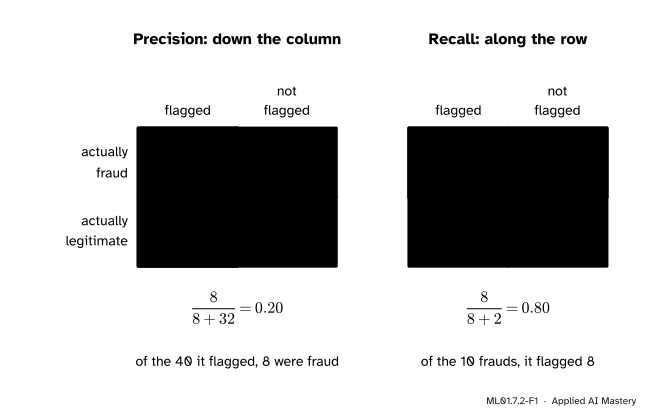
Model B of the last lesson, the detector, had \({\text{TP} = 8}\), \({\text{FN} = 2}\), \({\text{FP} = 32}\) and \({\text{TN} = 958}\).
ML01.7.2-F1
Two questions about the same table. Precision reads down the column of everything the model flagged. Recall reads along the row of everything that really was fraud. The greyed cells play no part.
Precision answers the first question: of the payments the model flagged, what share were fraud? Recall answers the second: of the payments that were fraud, what share did the model flag? Both have the true positives on top. They differ in what they divide by.
Build it up
Step 1. Precision reads down the column. The model flagged \({8 + 32 = 40}\) payments, and 8 of them were fraud. Precision is \({8/40 = 0.2}\). Four alarms in five are false.
Step 2. Recall reads along the row. There were \({8 + 2 = 10}\) frauds, and the model flagged 8. Recall is \({8/10 = 0.8}\).
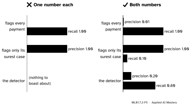
Step 3. Each one is blind to one mistake. Precision never looks at the false negatives. A model that flags only its single surest case, and is right, has precision \({1/1 = 1}\) while it misses nine frauds in ten. Recall never looks at the false positives. A model that flags every payment has recall \({10/10 = 1}\). Either number alone can be forced to 1, so report the pair.
Step 4. Neither one uses the true negatives. That is why they suit a rare positive class: the 958 legitimate payments rightly left alone are in neither formula.
Step 5. The threshold trades one for the other. Lower the threshold and the model flags no fewer examples. Every positive found before is still found, so recall never falls. But more negatives slip in too, and precision usually falls.
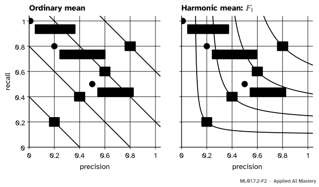
Step 6. One number, if you must. To rank models you may want a single score. The obvious one is the ordinary mean of precision and recall. Try it on three ways of flagging the payments:
Model
Precision, recall
Ordinary mean
Flags everything
\(0.01\), \(1\)
\(0.505\)
The detector
\(0.2\), \(0.8\)
\(0.5\)
A strict setting
\(0.5\), \(0.5\)
\(0.5\)
The ordinary mean ranks the model that flags everything first. A good score should be high only when both numbers are high. The harmonic mean does that; for precision and recall it is called the F1 score. For the three models it is \(0.02\), \(0.32\) and \(0.5\).
ML01.7.2-F2
Lines of equal score. Left: with the ordinary mean you can trade precision for recall one for one, all the way to the corner. Right: the lines of equal F1 bend away from the axes, so a model near either axis scores low.
Step 7. F1 still takes a side. It treats a false positive and a false negative as equally bad. If you know what each mistake costs, use the costs.
For the detector, \(F_1 = \frac{2 \times 0.2 \times 0.8}{0.2 + 0.8} = 0.32\).
Result 2: F1 from the counts. The reciprocals are simple, because both fractions have TP on top: \(\frac{1}{\text{prec}} = \frac{\text{TP} + \text{FP}}{\text{TP}}\) and \(\frac{1}{\text{rec}} = \frac{\text{TP} + \text{FN}}{\text{TP}}\). Half their sum is
All three scores are “hits over hits plus mistakes”. Precision counts the false positives as the mistakes, recall the false negatives, and F1 the average of the two. This form also works when \({\text{TP} = 0}\): then \({F_1 = 0}\).
Result 3: F1 is never more than twice the smaller number. Call the smaller of precision and recall \(m\) and the larger \(M\), so that \({F_1 = \frac{2mM}{m + M}}\). The bottom, \({m + M}\), is at least \(M\) and at most \(2M\). A larger bottom makes a smaller fraction, so
The model that flags everything has \({m = 0.01}\), so its F1 cannot pass \(0.02\), however good its recall is. The ordinary mean has no such limit: it is at least \(M/2\).
Result 4: F1 is never above the ordinary mean. Write \(a\) for precision and \(b\) for recall, and subtract:
The middle step uses \({(a + b)^2 - 4ab = a^2 - 2ab + b^2}\). The two means are equal only when \({a = b}\). For a given sum \({a + b}\), the gap grows with the square of \({a - b}\).
Choosing by cost. Suppose each false positive costs \(c_{\text{FP}}\) and each false negative costs \(c_{\text{FN}}\). Correct answers cost nothing. Then a model, at a given threshold, costs
and the best threshold is the one with the lowest cost on validation data. This puts the two mistakes on one scale chosen by you. F1 puts them on one scale chosen for you: equal weights.
Go deeper: F-beta: a harmonic mean that leans one way
A weighted harmonic mean can lean towards recall or towards precision. A number \(\beta\) sets the lean. Put in the counts, as in Result 2, and divide the top and the bottom by \({1 + \beta^2}\):
Like F1, this is hits over hits plus a weighted average of the mistakes. \({\beta = 1}\) gives equal weights: F1. With \({\beta = 2}\) a false negative counts four times as much as a false positive, which favours recall. With \({\beta = 0.5}\) it counts a quarter as much, which favours precision. For the detector, with \({\text{TP} = 8}\), \({\text{FN} = 2}\) and \({\text{FP} = 32}\),
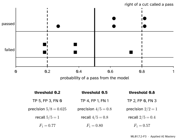
Part 1: the ten students at three thresholds. The probabilities are 0.182, 0.182, 0.378, 0.378 and 0.731 for the five fails, and 0.269, 0.622, 0.622, 0.818 and 0.818 for the five passes. “Pass” is the positive class.
ML01.7.2-F3
One model, three thresholds. Moving the cut to the right removes squares from the model’s passes, which lifts precision, and removes circles too, which lowers recall.
Threshold \(0.2\). Eight students are at or above it: all five passes and three fails. So \({\text{TP} = 5}\), \({\text{FP} = 3}\), \({\text{FN} = 0}\). Precision \({= 5/8 = 0.625}\), recall \({= 5/5 = 1}\), and by Result 2, \(F_1 = \frac{2 \times 5}{2 \times 5 + 3 + 0} = \frac{10}{13} = 0.769\).
Threshold \(0.8\). Only the two passes at \(0.818\) are called a pass. \({\text{TP} = 2}\), \({\text{FP} = 0}\), \({\text{FN} = 3}\). Precision \({= 2/2 = 1}\), recall \({= 2/5 = 0.4}\), and \({F_1 = \frac{4}{4 + 0 + 3} = \frac{4}{7} = 0.571}\).
Threshold
\(0.2\)
\(0.5\)
\(0.8\)
Precision
\(0.625\)
\(0.8\)
\(1\)
Recall
\(1\)
\(0.8\)
\(0.4\)
\(F_1\)
\(0.769\)
\(0.8\)
\(0.571\)
As the threshold rises, precision climbs from \(0.625\) to \(1\) and recall falls from \(1\) to \(0.4\). F1 is highest in the middle, where the two are balanced.
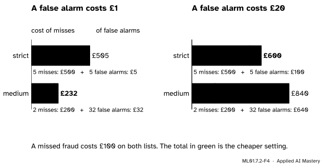
Part 2: choosing by cost. The payment detector can run at two settings. At the medium setting it is model B: \({\text{TP} = 8}\), \({\text{FP} = 32}\), \({\text{FN} = 2}\). At a strict setting it flags only 10 payments, 5 of them fraud: \({\text{TP} = 5}\), \({\text{FP} = 5}\), \({\text{FN} = 5}\). By Result 2 the F1 scores are \({\frac{16}{16 + 32 + 2} = 0.32}\) for medium and \({\frac{10}{10 + 5 + 5} = 0.5}\) for strict. F1 prefers strict.
Now put prices on the mistakes. Say a missed fraud costs £100. If a false alarm costs £1, a text message to the customer, then
The same two settings under two price lists. When alarms are cheap, catch more fraud. When they are dear, raise fewer of them.
The model and its F1 scores did not change. The price of a mistake did, and no metric can know that. When you can estimate the costs, let them choose the threshold.
Code
From scratch, from the four counts.
import numpy as npdef precision(tp, fp, fn):return tp / (tp + fp) if tp + fp >0elsefloat("nan") # undefined when nothing is flaggeddef recall(tp, fp, fn):return tp / (tp + fn)def f1(tp, fp, fn):return2* tp / (2* tp + fp + fn)def counts(y, said):"""(TP, FP, FN) with 1 as the positive class. True negatives are not needed.""" y, said = np.asarray(y), np.asarray(said)returnint(np.sum((y ==1) & (said ==1))), int(np.sum((y ==0) & (said ==1))), int(np.sum((y ==1) & (said ==0)))passed = np.array([0, 0, 0, 0, 0, 1, 1, 1, 1, 1])p = np.array([0.182, 0.182, 0.378, 0.378, 0.731, 0.269, 0.622, 0.622, 0.818, 0.818])for threshold in [0.2, 0.5, 0.8]: c = counts(passed, (p >= threshold).astype(int))print(f"threshold {threshold}: (TP, FP, FN) = {c} precision {precision(*c):.3f} "f"recall {recall(*c):.1f} F1 {f1(*c):.3f}")
The table of Part 1. Next, five ways of flagging the 1,000 payments, and the cost of two of them.
models = { # (TP, FP, FN) out of 10 frauds and 990 legitimate payments"flags everything": (10, 990, 0),"flags one sure case": (1, 0, 9),"strict setting": (5, 5, 5),"medium setting": (8, 32, 2),"flags nothing": (0, 0, 10),}for name, c in models.items(): pr, rc = precision(*c), recall(*c)print(f"{name:<20} precision {pr:.2f} recall {rc:.2f} ordinary mean {(pr + rc) /2:.3f} F1 {f1(*c):.3f}")def cost(c, per_alarm, per_miss=100): tp, fp, fn = creturn fp * per_alarm + fn * per_missfor per_alarm in [1, 20]:print(f"false alarm £{per_alarm}: strict £{cost(models['strict setting'], per_alarm)}, "f"medium £{cost(models['medium setting'], per_alarm)}")
flags everything     precision 0.01  recall 1.00  ordinary mean 0.505  F1 0.020
flags one sure case  precision 1.00  recall 0.10  ordinary mean 0.550  F1 0.182
strict setting       precision 0.50  recall 0.50  ordinary mean 0.500  F1 0.500
medium setting       precision 0.20  recall 0.80  ordinary mean 0.500  F1 0.320
flags nothing        precision nan  recall 0.00  ordinary mean nan  F1 0.000
false alarm £1: strict £505, medium £232
false alarm £20: strict £600, medium £840
The model that flags nothing has no precision: the cell prints nan for \(0/0\). Its F1, by the count formula, is \(0\).
The library version, on the last lesson’s detector of eights: 450 test images, 44 of them an 8. predict uses the threshold \(0.5\); for another threshold, compare predict_proba with it yourself.
At threshold \(0.5\) the detector is right in \(89\%\) of its alarms and finds \(73\%\) of the eights. Lowering the threshold to \(0.2\) finds three more eights, 35 instead of 32, at the price of seven more false alarms, 11 instead of 4. Recall rises to \(0.795\) and precision falls to \(0.761\). scikit-learn gives a model that flags nothing a precision of \(0\), with a warning unless you set zero_division.
Explore
This module’s interactive, the threshold slider, is in lesson 3. Press Rare (1 : 9) and slide the threshold slowly from left to right. Recall never rises, and precision mostly climbs. F1 rises, peaks and falls again. Press Jump to best F1: it lands at \(0.71\), not at \(0.5\).
Pitfalls
ML01.7.2-F5
Wrong beside right. Each useless model has one perfect number to show. Side by side, the pair gives them away.
“Precision is 1.00, so the model is excellent.”
Precision says nothing about what the model missed. Flag one sure case and precision is perfect while recall is \(0.1\). The same goes for recall: flag everything and it is \(1\). Never report one without the other.
“F1 is the average of precision and recall.”
It is their harmonic mean, which is never above the ordinary mean and is pulled towards the smaller number. For the model that flags everything, the ordinary mean is \(0.505\) and F1 is \(0.02\).
“The threshold with the best F1 is the best threshold.”
Only if a false positive and a false negative cost the same. In Part 2 the strict setting has the better F1 under both price lists, yet with cheap alarms the medium setting costs less than half as much. In machine learning the metric you optimise decides which model you ship, so choose it to match the costs.
“Precision and recall are properties of the model, whichever class I call positive.”
They belong to a model and a choice of positive class. For the detector with “fraud” as positive, precision is \(0.2\) and recall \(0.8\). Call “legitimate” positive instead and the same predictions give precision \({958/960 = 0.998}\) and recall \({958/990 = 0.968}\). Always say which class the numbers are for.
Check yourself
Recall
1. Write precision and recall in terms of the counts.
2. Which kind of mistake does precision ignore? Which does recall ignore?
Show answer
Precision ignores the false negatives, the positives that were missed. Recall ignores the false positives, the false alarms. Neither uses the true negatives.
3. How can a model with no skill reach a recall of 1?
Show answer
By flagging every example. Then nothing is missed, and the precision drops to the share of positives in the data.
4. Write F1 in terms of precision and recall, and in terms of the counts.
5. You lower the threshold. What happens to recall, and what usually happens to precision?
Show answer
Recall rises or stays the same. Precision usually falls, because more negatives are flagged too.
Exercises
1.★ A spam filter is tested on 200 emails. Its confusion matrix has \({\text{TP} = 45}\), \({\text{FP} = 15}\), \({\text{FN} = 5}\) and \({\text{TN} = 135}\). Compute its precision, recall and F1.
Show solution
Precision \({= \frac{45}{45 + 15} = 0.75}\): three quarters of the emails it marks are spam. Recall \({= \frac{45}{45 + 5} = 0.9}\): it catches nine spam emails in ten. \(F_1 = \frac{2 \times 45}{2 \times 45 + 15 + 5} = \frac{90}{110} = 0.818\).
2.★★ In Part 2 of the worked example a missed fraud costs £100. (a) At what cost of a false alarm do the strict and the medium setting cost the same? (b) A model that never flags anything misses all 10 frauds. Above what cost of a false alarm is it cheaper than both settings?
Show solution
(a) Let a false alarm cost \(c_{\text{FP}}\) pounds. Strict costs \({500 + 5c_{\text{FP}}}\) and medium costs \({200 + 32c_{\text{FP}}}\). They are equal when
Below £11.11 a false alarm, medium is cheaper. Above it, strict is.
(b) Never flagging misses all 10 frauds and costs £1,000. Strict costs more than that when \({5c_{\text{FP}} > 500}\), that is \({c_{\text{FP}} > 100}\). Medium costs more when \({32c_{\text{FP}} > 800}\), that is \({c_{\text{FP}} > 25}\). Both hold when \({c_{\text{FP}} > 100}\), so above £100 a false alarm it is cheapest to raise none. Strict raises one false alarm per fraud it catches, so it pays only while an alarm costs less than a missed fraud.
3.★★★ A model flags every example. (a) Show that its F1 is \({\frac{2\rho}{1 + \rho}}\), where \(\rho\) is the share of positives. (b) Evaluate it for the payments and for the ten students. What does this say about reading an F1 score?
Show solution
(a) Let there be \(P\) positives and \(N\) negatives, \({n = P + N}\) in all. Flagging everything gives \({\text{TP} = P}\), \({\text{FP} = N}\) and \({\text{FN} = 0}\). By Result 2,
So F1 has a do-nothing baseline too, which depends on the prevalence. On the balanced students, calling everyone a pass already scores \(0.667\), and the model’s \(0.8\) is only a little better. Like an accuracy, an F1 score means something only beside a baseline.
Summary card
Precision reads down the column, recall along the row, and F1 is high only when both are.
ML01.7.2-F1
Same hits, two different totals.
Precision.\({\frac{\text{TP}}{\text{TP} + \text{FP}}}\): of what the model flagged, the share that was right. Blind to misses.
Recall.\({\frac{\text{TP}}{\text{TP} + \text{FN}}}\): of the real positives, the share it found. Blind to false alarms.
F1.\(\frac{2 \cdot \text{prec} \cdot \text{rec}}{\text{prec} + \text{rec}} = \frac{2\,\text{TP}}{2\,\text{TP} + \text{FP} + \text{FN}}\), between the smaller number and twice the smaller.
Ten students. Thresholds \(0.2\), \(0.5\), \(0.8\): precision \(0.625\), \(0.8\), \(1\) and recall \(1\), \(0.8\), \(0.4\).
Cost.\(c_{\text{FP}} \cdot \text{FP} + c_{\text{FN}} \cdot \text{FN}\). When you know the prices, they choose the threshold.
Sources and next steps
Sources. Each was opened and checked against this lesson on 12 November 2026.
Daniel Jurafsky and James H. Martin, Speech and Language Processing, 3rd edition draft of 19 August 2026, Chapter 4, Section 4.9. Defines precision and recall, gives \({F_\beta = \frac{(\beta^2 + 1)PR}{\beta^2 P + R}}\) and \({F_1 = \frac{2PR}{P + R}}\) (equation 4.42), says that values of \(\beta\) above 1 favour recall, and explains the choice of mean: the harmonic mean of two values is closer to the smaller of them than the arithmetic mean is.
scikit-learn 1.9 User Guide, Metrics and scoring, Section 3.4.4.9 (precision, recall and F-measures). Calls the F-measure a weighted harmonic mean of precision and recall, and gives \(F_\beta\) in terms of tp, fp and fn; the “go deeper” note divides its top and bottom by \({1 + \beta^2}\).
Google, Machine Learning Crash Course, Accuracy, recall, precision, and related metrics. Gives the same formulas for precision and recall, and F1 as the harmonic mean, equal to \(\frac{2\,\text{TP}}{2\,\text{TP} + \text{FP} + \text{FN}}\).
Tom Fawcett, An introduction to ROC analysis, Pattern Recognition Letters 27 (2006), pages 861 to 874. Figure 1 of Section 2 lists precision, recall and the F-measure as \({2 / (1/\text{precision} + 1/\text{recall})}\). Section 6 treats the choice of an operating point from the costs of the two errors and the class proportions. Read in the copy hosted by the University of Houston.