Why a running average settles on the mean. Prove Markov’s and Chebyshev’s inequalities in a few lines, use them to prove the weak law of large numbers, and see what the law does not promise: no catching up after a streak.
Prove Markov’s inequality from the picture a·1{X ≥ a} ≤ X, and derive Chebyshev’s inequality from it.
State the weak law of large numbers and prove it from Chebyshev’s inequality and Var(X̄ₙ) = σ²/n.
Compute Chebyshev’s bound for a sample mean, compare it with the exact chance, and find the n that the bound guarantees.
Explain why relative frequencies in a simulation settle on probabilities, and why a streak is diluted rather than corrected.
In review. The maths and code on this page are checked by automated tests on every change, but an independent reader has not signed it off yet. Spot a mistake or a confusing step? Tell us.
The question
Every exact answer in this course has been checked by simulation: roll virtual dice many times and count. Lesson M06.1.3 promised that relative frequencies settle down. But a run of rolls is random, so why must its average settle anywhere, and how many rolls make it trustworthy? The same question sits under every Monte Carlo estimate (M07.10) and every average loss over a dataset.
From the last lesson
1. For i.i.d. draws with mean \(\mu\) and variance \(\sigma^2\), what are the expectation and the variance of the sample mean?
Show answer
\({\E[\bar{X}_n] = \mu}\) and \({\operatorname{Var}(\bar{X}_n)}\)\({= \sigma^2/n}\).
2. How much does the spread of an average shrink when the data are multiplied by four?
Show answer
It halves, because the standard deviation is \({\sigma/\sqrt{n}}\).
Intuition
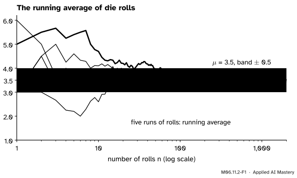
Roll a die again and again and keep the running average, the mean of all the rolls so far. Early on one roll moves it a lot. Later each new roll is one voice among hundreds and barely moves it.
M06.11.2-F1
Five runs of die rolls. Each path is the average of the rolls so far. They wander at first and then all settle into the band \({3.5 \pm 0.5}\), closer and closer to \({\mu = 3.5}\).
The last lesson explains the picture: the average of \(n\) rolls has spread \({\sigma/\sqrt{n}}\), which heads to zero. A spread near zero should mean “almost surely near the centre”. To turn that into a theorem we need one tool: a bound on how much probability can sit far from the mean, given only the variance.
Build it up
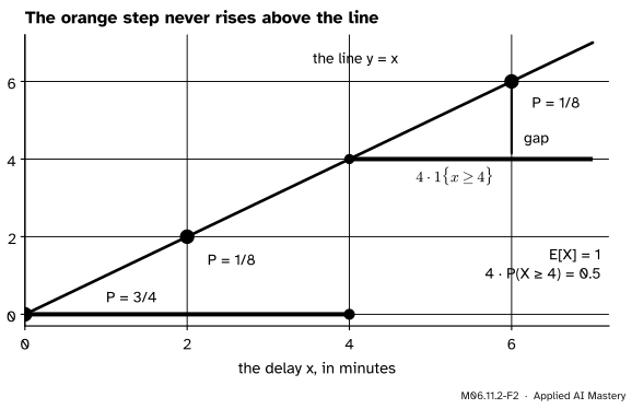
Step 1. Markov’s inequality. Take a variable that is never negative, such as the train delay of M06.7.4: 0, 2 or 6 minutes with chances \({3/4}\), \({1/8}\) and \({1/8}\), so \({\E[X] = 1}\). Pick a level, \({a = 4}\), and draw the step that is 0 below \(a\) and \(a\) from \(a\) on.
M06.11.2-F2
The step \({4 \cdot 1\{x \ge 4\}}\) (orange) never rises above the line \({y = x}\) when \({x \ge 0}\). So its average, \({4\,\Prob(X \ge 4)}\), cannot exceed the average of \(X\).
Here \({1\{X \ge a\}}\) is the indicator of the event \({X \ge a}\) (M06.7.1). Below \(a\) the step is 0, and \({X \ge 0}\). From \(a\) on the step is \(a\), and \({X \ge a}\). Either way
\[
a \cdot 1\{X \ge a\} \;\le\; X .
\]
Take expectations. The expectation of an indicator is the probability of its event, and a variable that is never larger has an expectation that is never larger:
\[
a\,\Prob(X \ge a) \;\le\; \E[X] .
\]
For the delay, \({\Prob(X \ge 4) \le 1/4}\). The exact chance is \({1/8}\): the bound is safe, not sharp.
Step 2. Chebyshev’s inequality. Apply Markov to the squared distance \({Y = (X - \mu)^2}\), which is never negative and has expectation \(\sigma^2\). For \({c > 0}\), the events \({\abs{X - \mu} \ge c}\) and \({Y \ge c^2}\) are the same, so
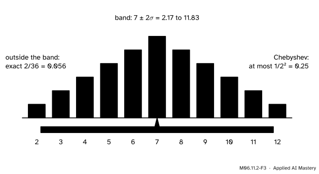
With \({c = k\sigma}\) this reads \({\Prob(\abs{X - \mu} \ge k\sigma)}\)\({\le 1/k^2}\): whatever the distribution, at most a quarter of the probability lies two standard deviations or more from the mean.
M06.11.2-F3
Chebyshev with \({k = 2}\) on the sum of two dice (\({\mu = 7}\), \({\sigma \approx 2.42}\)). Only the yellow bars lie outside \({7 \pm 2\sigma}\): exact chance \({2/36 \approx 0.056}\), well under the bound 0.25.
Step 3. Aim it at the average. The sample mean has mean \(\mu\) and variance \({\sigma^2/n}\). Put those into Chebyshev with \({c = \varepsilon}\), any tolerance we like.
The formal statement
NoteTheorem: the weak law of large numbers
Let \(X_1, X_2, \dots\) be i.i.d. with mean \(\mu\) and finite variance \(\sigma^2\). For every \({\varepsilon > 0}\),
and so \({\Prob(\abs{\bar{X}_n - \mu} \ge \varepsilon)}\)\({\to 0}\) as \({n \to \infty}\).
Proof. By the last lesson \({\E[\bar{X}_n] = \mu}\) and \({\operatorname{Var}(\bar{X}_n)}\)\({= \sigma^2/n}\). Chebyshev’s inequality for the variable \(\bar{X}_n\) with \({c = \varepsilon}\) gives
For a fixed \(\varepsilon\) the right-hand side is a constant divided by \(n\), so it goes to 0. A probability lies between 0 and something that goes to 0, so it goes to 0 too. \(\square\)
In words: pick any band around \(\mu\), however narrow. The chance that the average lies outside it can be made as small as you like by taking enough draws.
Frequencies are averages. Let \({X_i = 1}\) when an event \(A\) happens on trial \(i\) and 0 otherwise. Then \(\bar{X}_n\) is the relative frequency of \(A\), with mean \({p = \Prob(A)}\) and variance \({p(1 - p)/n}\). The law says the frequency settles on the probability, which is why the course’s simulations work. Since \({p(1 - p) \le 1/4}\), the bound is at most \({1/(4n\varepsilon^2)}\) whatever \(p\) is.
Go deeper: weak, strong, and the case without a variance
The weak law speaks about one \(n\) at a time: for large \(n\), a miss by \(\varepsilon\) is unlikely. The strong law says more about a whole run: with probability 1, the running average converges to \(\mu\). The variance was a convenience of this proof. The weak law holds for any i.i.d. sequence with a finite mean, but that proof needs more tools; both are in M07.5. A mean is needed: for the Cauchy distribution, which has none, the average of \(n\) draws is as spread out as one draw, and the running average never settles (M06.11.3).
Worked example
How many dice for a mean within 0.5 of 3.5? For a die \({\sigma^2 = 35/12}\). With \({\varepsilon = 0.5}\) the bound is
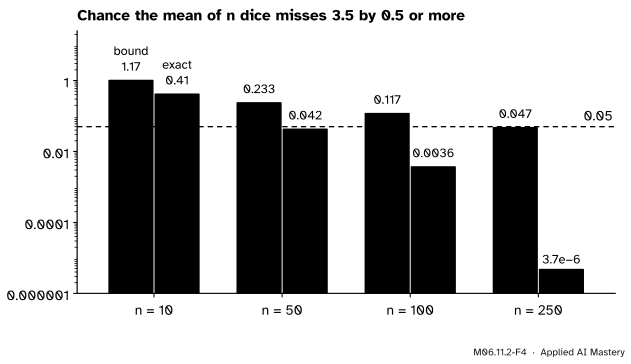
At \({n = 10}\) it is \({35/30 \approx 1.17}\): true, but useless, since every probability is at most 1. At \({n = 100}\) it is 0.117. To guarantee a miss chance of at most 0.05 we need \({35/(3n) \le 0.05}\), that is \({n \ge 700/3 \approx 233.3}\), so \({n = 234}\) dice.
M06.11.2-F4
Chebyshev’s bound (vermillion) beside the exact chance (grey), from convolving \(n\) dice. The bound falls like \(1/n\); the truth falls far faster. Note the log scale.
The exact chances come from the exact distribution of the mean (convolution, as in the last lesson). At \({n = 100}\) the truth is 0.0036, about 32 times smaller than the bound. Chebyshev knows only \(\mu\) and \(\sigma\), so it must hold for the worst distribution with those two numbers. The central limit theorem of the next lesson uses the shape of the average and gives estimates close to the truth.
Code
First the two inequalities, exactly, with fractions.
from fractions import Fraction as Fdelay = {0: F(3, 4), 2: F(1, 8), 6: F(1, 8)} # the train delayE =lambda pmf, g=lambda x: x: sum(g(x) * p for x, p in pmf.items())print("Markov: P(X >= 4) =", sum(p for x, p in delay.items() if x >=4), "<= E[X]/4 =", E(delay) /4)two = {s: F(6-abs(s -7), 36) for s inrange(2, 13)} # sum of two dicevar2 = E(two, lambda s: (s -7) **2)outside =sum(p for s, p in two.items() if (s -7) **2>=4* var2) # |S - 7| >= 2 sigmaprint("Chebyshev: P(|S - 7| >= 2 sigma) =", outside, "<= 1/4; Var(S) =", var2)
Next, the worked example: the bound against the exact chance from repeated convolution.
import numpy as npdef miss_chance(n, eps=0.5): pmf = np.array([1.0])for _ inrange(n): pmf = np.convolve(pmf, np.full(6, 1/6)) means = np.arange(n, 6* n +1) / nreturn pmf[np.abs(means -3.5) >= eps -1e-12].sum()for n in (10, 50, 100, 250):print(f"n = {n:3}: Chebyshev {35/ (3* n):.3f} exact {miss_chance(n):.2g}")print("smallest n with bound <= 0.05:", int(np.ceil(35/ (3*0.05))))
n =  10: Chebyshev 1.167   exact 0.41
n =  50: Chebyshev 0.233   exact 0.042
n = 100: Chebyshev 0.117   exact 0.0036
n = 250: Chebyshev 0.047   exact 3.7e-06
smallest n with bound <= 0.05: 234
Finally the law at work in a simulation: running averages with numpy.cumsum, and the frequency of a sum of 7 settling on \({1/6}\).
rng = np.random.default_rng(1)rolls = rng.integers(1, 7, size=10_000)running = np.cumsum(rolls) / np.arange(1, 10_001)print("running average after 10, 100, 10,000 rolls:", running[[9, 99, 9_999]].round(3))sevens = (rng.integers(1, 7, size=10_000) + rng.integers(1, 7, size=10_000)) ==7print("share of sevens in 10,000 throws:", sevens.mean(), " exact 1/6 =", round(1/6, 4))print("Chebyshev bound for missing 1/6 by 0.01:", round((1/6) * (5/6) / (10_000*0.01**2), 3))
running average after 10, 100, 10,000 rolls: [3.5   3.51  3.501]
share of sevens in 10,000 throws: 0.1703   exact 1/6 = 0.1667
Chebyshev bound for missing 1/6 by 0.01: 0.139
The simulated numbers will differ in the last digits on another machine; the bound of 0.139 does not, and it says a miss by 0.01 or more happens in at most about one run of 10,000 throws in seven.
Explore
The sample-mean machine is in lesson M06.11.3. Choose the skewed source and draw a few hundred means at \({n = 2}\), then at \({n = 50}\). The read-out counts how many of your means lie within two spreads of \(\mu\); watch the whole histogram crowd into a narrower and narrower strip around \(\mu\) as \(n\) grows.
Pitfalls
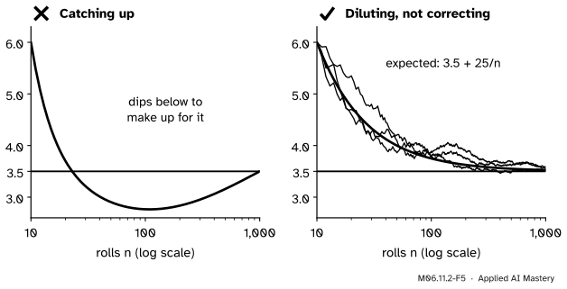
M06.11.2-F5
Wrong beside right, after ten sixes in a row. The average does not dip below 3.5 to make up for the streak (left). The streak is diluted by new rolls: the expected average is \({3.5 + 25/n}\) (right).
“After a run of sixes, low rolls are due, so the average can come back.”
The dice have no memory: the rolls after the streak are independent of it. After 10 sixes the total is 60, and each later roll adds 3.5 on average, so after \(n\) rolls
The extra 25 in the total is never paid back; it is spread over more and more rolls. This mistaken belief is called the gambler’s fallacy.
“For large n the total equals n times the mean.”
The average closes in on \(\mu\), but the total\({S_n}\) does not close in on \({n\mu}\): its spread \({\sigma\sqrt{n}}\) grows. After 10,000 rolls the total typically misses 35,000 by about \({1.71 \times 100 = 171}\), while the average misses 3.5 by only about 0.017.
“Chebyshev’s bound is the probability.”
It is a ceiling that holds for every distribution with the same mean and variance, so it is often far above the truth: 0.117 against 0.0036 for 100 dice. Use it for guarantees, not estimates. Sharper bounds (M07.6) use more than the variance.
Check yourself
Recall
1. State Markov’s inequality and the condition it needs.
Show answer
For a variable that is never negative and any \({a > 0}\), \({\Prob(X \ge a) \le \E[X]/a}\).
2. State Chebyshev’s inequality with \(k\) standard deviations.
Show answer
\({\Prob(\abs{X - \mu} \ge k\sigma)}\)\({\le 1/k^2}\) for any variable with finite variance.
3. State the weak law of large numbers with the bound from the proof.
Show answer
For i.i.d. draws with mean \(\mu\) and variance \(\sigma^2\), \({\Prob(\abs{\bar{X}_n - \mu} \ge \varepsilon)}\)\({\le \sigma^2/(n\varepsilon^2)}\), which goes to 0 as \(n\) grows.
4. Why does a simulated relative frequency settle on a probability?
Show answer
It is the sample mean of indicators, whose mean is the probability \(p\) and whose variance is \({p(1 - p)}\); the law of large numbers applies.
5. After ten sixes, what is the expected average after \(n\) rolls in all?
Show answer
\({3.5 + 25/n}\): the streak is diluted, never corrected.
Exercises
1.★ A waiting time has mean 2 minutes. Without knowing anything else, bound the chance that it is at least 10 minutes.
Show solution
A waiting time is never negative, so Markov gives \({\Prob(T \ge 10) \le 2/10 = 0.2}\). (For the exponential waiting time of the course the exact value is \({e^{-0.5 \times 10}}\)\({= e^{-5}}\)\({\approx 0.0067}\).)
2.★★ You simulate a fair coin to estimate \({\Prob(\text{heads}) = 0.5}\). Use Chebyshev to find how many flips guarantee a chance of at most 0.01 that the frequency misses 0.5 by 0.05 or more.
Show solution
The frequency has variance \({0.25/n}\), so the bound is \({0.25/(n \times 0.05^2) = 100/n}\). We need \({100/n \le 0.01}\), so \({n \ge 10{,}000}\) flips.
3.★★★ Show that Chebyshev’s inequality can be an equality. Take \(X\) equal to \(-c\) or \(c\) with chance one half each, and compute both sides for \({k = 1}\).
Show solution
\({\mu = 0}\) and \({\sigma^2 = c^2}\), so \({\sigma = c}\). The event \({\abs{X - 0} \ge 1 \cdot \sigma}\) is \({\abs{X} \ge c}\), which always happens, so the left side is 1. The right side is \({1/1^2 = 1}\). So no better general bound is possible with \({k = 1}\); for \({k > 1}\), put probability \({1/(2k^2)}\) at each of \({\pm k}\) and the rest at 0 to get equality.
Summary card
Averages settle on the mean, because their spread goes to zero.
M06.11.2-F1
Running averages close in on \(\mu\).
Markov:\({\Prob(X \ge a) \le \E[X]/a}\) for \({X \ge 0}\).
Frequencies settle on probabilities; a streak is diluted, not corrected.
Sources and next steps
Sources. Each was opened and checked against this lesson on 12 November 2026.
Hossein Pishro-Nik, Markov and Chebyshev Inequalities, Section 6.2.2, both inequalities with their proofs (Chebyshev by Markov applied to \({(X - \E X)^2}\)), and Law of Large Numbers, Section 7.1.1, the weak law proved from Chebyshev with the bound \({\operatorname{Var}(X)/(n\varepsilon^2)}\), in Introduction to Probability, Statistics, and Random Processes.
Charles M. Grinstead and J. Laurie Snell, Introduction to Probability, second edition, Section 8.1: Theorem 8.1 (Chebyshev), Example 8.1 (the form \({1/k^2}\)), the remark after it (a two-point distribution for which the inequality is an equality) and Theorem 8.2 (the law of large numbers).
Jeremy Orloff and Jonathan Bloom, Reading 6b: Central Limit Theorem and the Law of Large Numbers, MIT OpenCourseWare 18.05, Spring 2022. Section 3 follows the share of heads in \(n\) flips (the chance of lying within 0.1 of 0.5 rises from 0.656 at \({n = 10}\) to 0.965 at \({n = 100}\)); Section 3.1 states the law formally.