Turn the central limit theorem into numbers: approximate probabilities for sums and means by standardising and reading Φ, with the continuity correction for counts, the mean ± 2 standard deviations range, and the cases where the bell is a poor guide.
Approximate a probability for a sum or a mean of i.i.d. draws by standardising it and reading Φ.
Apply the continuity correction to an integer-valued sum and explain it with the picture of bars as areas.
Use mean ± 2 standard deviations as a range that holds about 95% of the time, for test accuracy and for mini-batch gradients.
Recognise when the approximation is poor: small n, p near 0 or 1, heavy tails, and check it against scipy.stats.binom.
In review. The maths and code on this page are checked by automated tests on every change, but an independent reader has not signed it off yet. Spot a mistake or a confusing step? Tell us.
The question
A coin lands heads 60 times in 100 flips. Is that surprising for a fair coin? A model scores 0.85 on 100 test examples when you believed its accuracy was 0.9: bad luck, or a real drop? Both need the chance of a sum landing far from its mean. Exact answers need the whole distribution; the central limit theorem gives a good answer from just the mean and the standard deviation.
From the last lesson
1. State the central limit theorem.
Show answer
For i.i.d. draws with mean \(\mu\) and finite variance \({\sigma^2 > 0}\), \({\Prob(Z_n \le z) \to \Phi(z)}\), where \({Z_n}\)\({= (\bar{X}_n - \mu)/(\sigma/\sqrt{n})}\).
2. Why do averages of Cauchy draws never approach a bell?
Show answer
The Cauchy distribution has no finite variance; the average of \(n\) draws has the same distribution as one draw.
Intuition
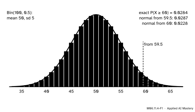
The number of heads in 100 fair flips is \({\mathrm{Bin}(100, 0.5)}\): a sum of 100 Bernoulli variables, with mean 50 and standard deviation \({\sqrt{100 \times 0.25} = 5}\). The central limit theorem says its bars should follow the normal curve with that mean and spread.
M06.11.4-F1
\({\Prob(X \ge 60)}\) as the yellow bars (exact) and as the area under the normal curve (vermillion). Starting the area at 59.5, the left edge of the bar for 60, gets within 0.0003 of the truth.
Every bar has width 1, so its area is its probability. “60 or more” is the yellow bars, and the curve’s area over the same stretch of axis, from 59.5 onwards, is nearly the same. Getting that area is one call to \(\Phi\).
Build it up
Step 1. Centre and spread of the sum. For a sum of \(n\) i.i.d. draws, \({\E[S_n] = n\mu}\) and \({\sigma_{S_n} = \sigma\sqrt{n}}\). For the flips, \({\mu = 0.5}\) and \({\sigma = 0.5}\), giving 50 and 5.
Step 2. Mind the bars.\(X\) takes whole values only, so “60 or more” and “more than 59.5” are the same event. On the picture, the bar for 60 starts at 59.5.
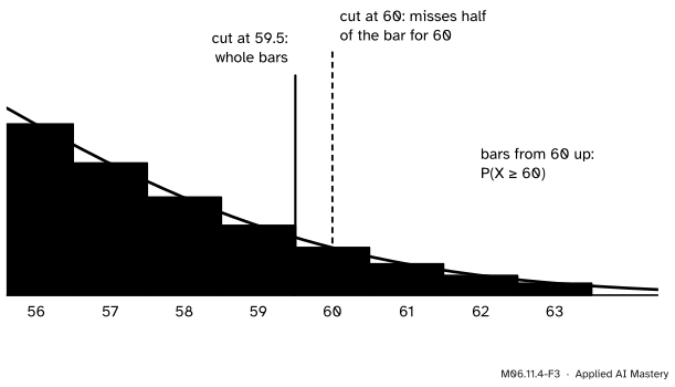
Why the half. Picture each value \(k\) as a bar of width 1 from \({k - 0.5}\) to \({k + 0.5}\). The exact \({\Prob(S_n \ge k)}\) is the area of the bars from \(k\) up, which start at \({k - 0.5}\), so we take the curve’s area from there too. Cutting at \(k\) itself drops half of the bar for \(k\).
M06.11.4-F3
The bar for 60 spans 59.5 to 60.5. Cutting the curve at 60 (dashed) leaves out half of it, which is why 0.0228 falls short of the exact 0.0284.
Go deeper: a mean, a skewed source and a lattice of step 2
Take the average of 50 train delays (0, 2 or 6 minutes; \({\mu = 1}\), \({\sigma = 2}\)) and ask for \({\Prob(\bar{X}_{50} > 1.5)}\), that is \({S_{50} > 75}\). The sum takes only even values, so its bars have width 2 and the half-way point between 74 and 76 is 75 itself: the cut needs no shift. Then \({z}\)\({= (75 - 50)/(2\sqrt{50})}\)\({\approx 1.768}\) and the bell gives \({1 - \Phi(1.768) \approx 0.039}\). The exact value, from 50 convolutions, is 0.046. The gap is the leftover skewness, \({1.875/\sqrt{50} \approx 0.27}\): a right-skewed source keeps a fatter right tail than the bell, so the approximation is too small there.
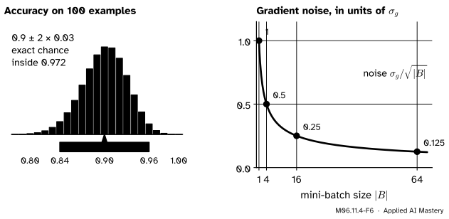
A 95% range. Since \({\Phi(2) - \Phi(-2) \approx 0.954}\), a sum or mean lands within two standard deviations of its centre about 95% of the time. (\({\pm 1.96}\) gives 0.950 exactly.) For accuracy on 100 test examples at true accuracy 0.9 that is \({0.9 \pm 2 \times 0.03 = 0.9 \pm 0.06}\), from 0.84 to 0.96. A score of 0.85 is inside the range, so bad luck explains it.
M06.11.4-F6
Left: the range \({0.9 \pm 0.06}\) for a test score, which holds with exact chance 0.972. Right: the noise in a mini-batch gradient falls like \({1/\sqrt{\abs{B}}}\).
Mini-batch gradients. Stochastic gradient descent (ML01.5.4) averages the gradients of a mini-batch \(B\) of \(\abs{B}\) examples drawn at random. If the examples are drawn independently and one example’s gradient has standard deviation \(\sigma_g\), the mini-batch average has standard deviation \({\sigma_g/\sqrt{\abs{B}}}\), and for a batch of more than a few examples it is close to normal. Going from 1 to 64 examples cuts the noise by 8, not by 64. (Drawing the batch without replacement from a finite dataset makes the noise slightly smaller still, as ML01.5.4 shows.)
Worked example
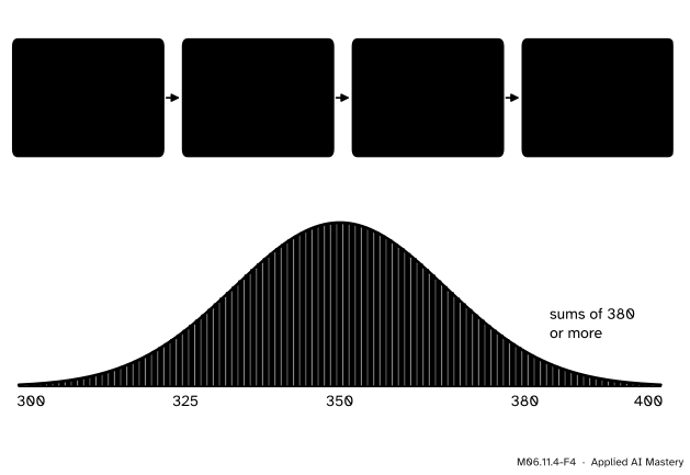
The sum of 100 dice. Find \({\Prob(S \ge 380)}\).
The centre is \({100 \times 3.5 = 350}\). The standard deviation is \({\sqrt{100} \times \sqrt{35/12}}\)\({\approx 10 \times 1.708}\)\({= 17.08}\). The sum is whole-valued, so “380 or more” starts at 379.5:
The worked example as a trace. The exact distribution of the sum (below), from 100 convolutions, is almost exactly the normal curve, and the tail from 380 matches to four decimals.
The exact value, from convolving 100 dice, is 0.0420. Without the correction, \({1 - \Phi(30/17.08) \approx 0.0395}\), off by 0.0025 where the corrected value is off by 0.00002. A sum of 380 or more happens in about one batch of 100 rolls in 24.
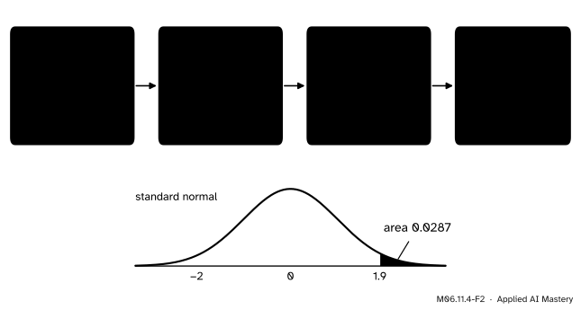
Back to the question: 0.85 on 100 test examples. If the true accuracy is 0.9, the number correct \(X\) has mean 90 and standard deviation 3. A score of 0.85 or lower means \({X \le 85}\), which ends at 85.5:
The exact binomial value is 0.073. So a model whose accuracy has not changed at all scores 0.85 or less on about one test set in 14. One such score is weak evidence of a real drop; a larger test set, or a second one, is the honest next step. Here \(p\) is near 1, so the counts are a little skewed and the bell is less accurate than for the fair coin, but it still tells the right story.
Code
From scratch, with \(\Phi\) from math.erf, against exact answers.
import mathimport numpy as npdef Phi(z):return0.5* (1+ math.erf(z / math.sqrt(2)))def normal_tail(k, n, mu, sigma, correct=True):"""Approximate P(S_n >= k) for a whole-valued sum of n i.i.d. draws.""" cut = k -0.5if correct else kreturn1- Phi((cut - n * mu) / (sigma * math.sqrt(n)))dice = np.array([1.0])for _ inrange(100): dice = np.convolve(dice, np.full(6, 1/6)) # exact PMF of the sum, values 100 to 600exact_dice = dice[380-100:].sum()print(f"100 dice, S >= 380: exact {exact_dice:.4f} corrected {normal_tail(380, 100, 3.5, math.sqrt(35/12)):.4f}"f" uncorrected {normal_tail(380, 100, 3.5, math.sqrt(35/12), False):.4f}")exact_heads =sum(math.comb(100, k) for k inrange(60, 101)) /2**100print(f"100 flips, X >= 60: exact {exact_heads:.4f} corrected {normal_tail(60, 100, 0.5, 0.5):.4f}"f" uncorrected {normal_tail(60, 100, 0.5, 0.5, False):.4f}")
The same with scipy. norm takes the standard deviation as scale, not the variance; binom.sf(k, n, p) is \({\Prob(X > k)}\), so “60 or more” is sf(59, ...).
Last, mini-batch noise. A line \({y = 2x + \text{noise}}\) is fitted by squared error with weight \({w = 0}\), so one example’s gradient is \({-2xy}\). Its standard deviation works out to \({\sigma_g = 6}\) (an exercise below), so a batch of \(\abs{B}\) examples should give \({6/\sqrt{\abs{B}}}\). In the code, B holds the batch size.
rng = np.random.default_rng(0)for B in (1, 4, 16, 64): x = rng.normal(size=(20_000, B)) y =2* x + rng.normal(size=(20_000, B)) grads = (-2* x * y).mean(axis=1) # 20,000 mini-batch gradientsprint(f"B = {B:2}: sd of the batch gradient {grads.std():.2f} 6/sqrt(B) = {6/ math.sqrt(B):.2f}")
B =  1: sd of the batch gradient 5.93   6/sqrt(B) = 6.00
B =  4: sd of the batch gradient 3.02   6/sqrt(B) = 3.00
B = 16: sd of the batch gradient 1.50   6/sqrt(B) = 1.50
B = 64: sd of the batch gradient 0.75   6/sqrt(B) = 0.75
Explore
Use the sample-mean machine in lesson M06.11.3 as a check on the 95% range. Pick the die, set \({n = 50}\), and draw several hundred means with the normal curve on. The read-out reports the share of your means within two spreads of \(\mu\); it should be close to 0.954 (the exact share for 50 dice is 0.958, since the means sit on a lattice). Then pick the coin with \({p = 0.05}\) and \({n = 10}\): only 0.5 heads are expected per sample, the means pile up at 0, the curve spills below 0, and the exact share within two spreads falls to 0.914. The read-out warns that the bell fits badly.
Pitfalls
M06.11.4-F5
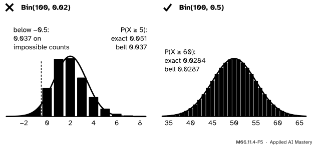
Wrong beside right. With \({p = 0.02}\) the counts are skewed and pressed against 0, and the bell both spills onto negative counts and thins the right tail. With \({p = 0.5}\) it fits.
“With n = 100 the bell is always fine.”
It depends on \({np(1 - p)}\), not on \(n\) alone. \({\mathrm{Bin}(100, 0.02)}\) has mean 2 and standard deviation 1.4: the bell puts 0.037 of its probability below \({-0.5}\), on impossible negative counts, and gives \({\Prob(X \ge 5) \approx 0.037}\) against the exact 0.051. For rare events use the exact binomial (or the Poisson of M06.8.3). The same goes for a very small \(n\), and for heavy tails, where the bell can fail outright (M06.11.3).
“Cut at 60 for 60 or more.”
For a whole-valued count that drops half a bar: 0.0228 instead of 0.0284 for 60 or more heads, about a fifth too small. Cut half-way between values: at 59.5 for “60 or more”, at 60.5 for “60 or fewer”.
“scipy’s norm takes the variance.”
stats.norm(loc, scale) takes the standard deviation as scale. Passing the variance 291.7 for 100 dice instead of 17.08 makes the curve 17 times too wide, and every tail probability far too big.
Check yourself
Recall
1. Give the normal approximation to \({\Prob(S_n \le s)}\).
Show answer
\({\Phi\big((s - n\mu)/(\sigma\sqrt{n})\big)}\).
2. What is the continuity correction for \({\Prob(S_n \ge k)}\) when \(S_n\) is whole-valued?
Show answer
Cut at \({k - 0.5}\): with \({z = (k - 0.5 - n\mu)/(\sigma\sqrt{n})}\), the chance is about \({1 - \Phi(z)}\).
3. What range holds a sum or mean about 95% of the time?
Show answer
Its centre plus or minus two standard deviations (\({\pm 1.96}\) for 0.950).
4. How does the noise in a mini-batch gradient depend on the batch size \(\abs{B}\)?
Show answer
Its standard deviation is \({\sigma_g/\sqrt{\abs{B}}}\), for examples drawn independently.
5. Name two situations where the normal approximation is poor.
Show answer
Any two of: small \(n\); \(p\) near 0 or 1, so \({np(1 - p)}\) is small; heavy tails with no finite variance.
Exercises
1.★ Approximate the chance of 45 or fewer heads in 100 fair flips, with the continuity correction.
Show solution
“45 or fewer” ends at 45.5, so \({z = (45.5 - 50)/5 = -0.9}\) and the chance is about \({\Phi(-0.9) \approx 0.184}\). (Exact: 0.184.)
2.★★ A model with true accuracy 0.8 is tested on 400 examples. Give the range that holds the measured accuracy about 95% of the time.
Show solution
The standard deviation is \({\sqrt{0.8 \times 0.2/400}}\)\({= 0.4/20}\)\({= 0.02}\), so the range is \({0.8 \pm 0.04}\), from 0.76 to 0.84.
3.★★★ In the mini-batch example, \(x\) and the noise \(\varepsilon\) are independent \({N(0, 1)}\) and \({y = 2x + \varepsilon}\). Show that one gradient \({g = -2xy}\) has mean \(-4\) and standard deviation 6. Use \({\E[x^2] = 1}\) and \({\E[x^4] = 3}\).
So \({\operatorname{Var}(g)}\)\({= 52 - (-4)^2}\)\({= 36}\) and \({\sigma_g = 6}\).
Summary card
Standardise, mind the bars, read Φ.
M06.11.4-F1
Bars as areas under the bell.
\({z = (s - n\mu)/(\sigma\sqrt{n})}\), then \({\Prob(S_n \le s) \approx \Phi(z)}\).
Whole values: cut at \({k \pm 0.5}\). Heads \({\ge 60}\) of 100: 0.0287 (exact 0.0284).
95% range: centre \({\pm 2}\) sd. Accuracy 0.9 on 100: \({0.9 \pm 0.06}\).
Gradient noise \({\sigma_g/\sqrt{\abs{B}}}\). Poor for small \(n\), \(p\) near 0 or 1, heavy tails.
Sources and next steps
Sources. Each was opened and checked against this lesson on 12 November 2026.
Hossein Pishro-Nik, Central Limit Theorem, Section 7.1.2 of Introduction to Probability, Statistics, and Random Processes: the continuity correction for an integer-valued sum, \({\Prob(l \le Y \le u)}\)\({= \Prob(l - \tfrac12 \le Y \le u + \tfrac12)}\), with a worked binomial example where it improves the estimate.
Jeremy Orloff and Jonathan Bloom, Reading 6b: Central Limit Theorem and the Law of Large Numbers, MIT OpenCourseWare 18.05, Spring 2022. Section 5.3 (the probabilities within 1, 2 and 3 standard deviations) and Section 5.4 (approximating heads in 100 flips, including 40 to 60 heads: 0.954 by the theorem against 0.965 exactly).
Chris Piech, Central Limit Theorem, Probability for Computer Scientists: the sum of dice approximated by a normal with the continuity correction.
SciPy, scipy.stats.norm (loc is the mean and scale the standard deviation; sf is \({1 - \text{cdf}}\)) and scipy.stats.binom (shape parameters n and p, and sf).
Next. This closes Probability I. S02.1 studies sampling distributions in general, and S02.4 turns the 95% range around into a confidence interval for an unknown mean.