Before anything can have a probability, you must list what could happen. Learn to name an experiment, its outcomes and its sample space, to list them for coins and dice, and to tell finite, countably infinite and continuous sample spaces apart.
Name the experiment, its outcomes and its sample space for a chance situation, and write the sample space as a set.
List the sample space of a coin, a die, three coin flips and two dice, and count it with the multiplication rule or by adding branches.
Tell a finite sample space from a countably infinite one and from a continuous one.
Choose outcomes fine enough to answer a question, and build the sample space in Python with itertools.product.
In review. The maths and code on this page are checked by automated tests on every change, but an independent reader has not signed it off yet. Spot a mistake or a confusing step? Tell us.
The question
Roll two dice. How many different things can happen: 11 possible sums, 21 pairs of faces, or 36 ordered pairs? All three lists are honest descriptions of the same roll, yet only one of them lets you answer every question about it, and only one of them has outcomes that are all equally likely. Which one, and how do you decide before you compute a single probability?
Intuition
Probability always starts with a list. Before you can say how likely something is, you must say what could happen at all.
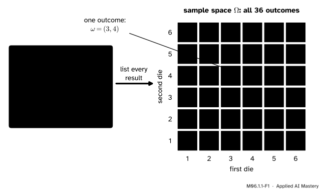
An experiment is any procedure whose result is uncertain and that could, at least in principle, be repeated: roll two dice, flip a coin three times, draw a mini-batch of examples, spin a spinner. An outcome is one complete result of the experiment. The sample space, written \(\Omega\) (the Greek capital omega), is the set of all the outcomes. A single outcome is written \(\omega\), a small omega.
M06.1.1-F1
The course’s running example. The experiment is a roll of two dice; one outcome is the ordered pair (first die, second die), and the sample space \(\Omega\) is the grid of all 36 such pairs.
Think of the sample space as the menu that chance orders from. Each time the experiment runs, exactly one item on the menu comes up. Two rules make a list a proper sample space:
Nothing is left out. Whatever happens, it is on the list.
No two items overlap. Whatever happens, it matches exactly one item.
The two dice are painted different colours in the picture so that you can always tell which is the first. Then a 3 on the first and a 4 on the second, \({(3, 4)}\), is a different result from \({(4, 3)}\). That is why the grid has 36 cells and not fewer.
Build it up
We build sample spaces for four experiments, each a little richer than the last.
Step 1. One coin. The outcomes are heads and tails, so \({\Omega = \{H, T\}}\). A set has no order, so \({\{T, H\}}\) is the same sample space (sets were met in M01.6).
Step 2. One die.\({\Omega = \{1, 2, 3, 4, 5, 6\}}\). The number of outcomes is written \({|\Omega|}\), as for any finite set, so here \({|\Omega| = 6}\).
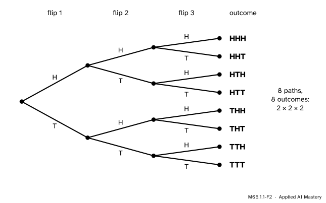
Step 3. Three coin flips. One outcome must record all three flips, in order, such as HTH. A tree builds the list: each flip splits every branch in two.
M06.1.1-F2
Three flips as a tree. Every path from the root to a leaf is one outcome, so the eight leaves are the eight outcomes, from HHH to TTT.
The multiplication rule of counting (M01.8) gives the size without drawing anything: two choices, then two, then two, so \({|\Omega| = 2 \times 2 \times 2 = 8}\).
Step 4. Two dice. An outcome is an ordered pair \({(i, j)}\), with \(i\) the first die and \(j\) the second. The sample space is the set of all such pairs, the grid of the anchor picture, and \({|\Omega| = 6 \times 6 = 36}\).
Step 5. When the list never ends. Flip a coin until the first head appears. The outcomes are H, TH, TTH, TTTH and so on: no last outcome exists, because any number of tails can come first. Yet the outcomes can still be numbered 1, 2, 3, …, by the flip on which the head arrives.
Step 6. When the outcomes cannot be listed at all. Spin a spinner and read where it stops, as a fraction of a full turn. Every number from 0 up to (but not including) 1 is possible, so \({\Omega = [0, 1)}\), an interval of real numbers.
The formal statement
NoteDefinition: sample space
A random experiment is a procedure, repeatable in principle, whose result is uncertain. The sample space\(\Omega\) is a set whose elements, the outcomes\(\omega\), are the possible results, chosen so that each run of the experiment produces exactly one outcome.
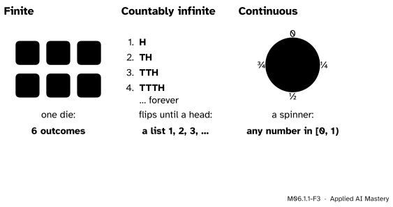
“Exactly one” packs both rules of the intuition: at least one (nothing is left out) and at most one (no overlaps). The sample spaces of this course come in three kinds.
M06.1.1-F3
Three kinds of sample space. A finite one can be listed and counted. A countably infinite one can be listed but the list never ends. A continuous one cannot be listed at all.
Finite.\(\Omega\) has a whole number of outcomes, \({|\Omega|}\). A die, three flips, two dice.
Countably infinite. The outcomes can be put in a list \({\omega_1, \omega_2, \omega_3, \dots}\) that never ends but reaches every outcome sooner or later. Flips until the first head, or the number of emails that arrive in an hour.
Continuous. The outcomes fill an interval of real numbers, or a region, and no list can reach them all. The spinner, a waiting time, a measured height.
Finite and countably infinite spaces are called discrete. The modules up to M06.5 work with discrete spaces; continuous ones return in M06.6, where probabilities become areas under curves.
Go deeper: why no list can hold every point of the spinner
Suppose someone claims a list \({x_1, x_2, x_3, \dots}\) that contains every number in \({[0, 1)}\). Write each number as a decimal, and build a new number \(y\), one digit at a time: the \(k\)-th digit of \(y\) is 5 if the \(k\)-th digit of \(x_k\) is not 5, and 4 if it is.
Then \(y\) lies in \({[0, 1)}\) and differs from \(x_k\) in the \(k\)-th digit, for every \(k\). Because \(y\) uses only the digits 4 and 5, it has just one decimal form (the trouble case, a tail of 9s such as 0.4999… = 0.5, cannot arise), so differing in a digit really means being a different number. So \(y\) is missing from the list, and no list can be complete. This is Cantor’s diagonal argument.
Building a sample space in stages. When an experiment runs in stages and every stage has the same choices whatever happened before, an outcome is a tuple with one entry per stage, and \(\Omega\) is the Cartesian product of the stages’ choices. For two dice,
When the choices at a later stage depend on what happened earlier, the product rule no longer applies. Then list the branches and add, as the worked example shows.
Fine enough to answer the question. A sample space is a choice, and the same experiment has several honest ones. For two dice you could record only the sum, \({\{2, 3, \dots, 12\}}\), with 11 outcomes. That space can answer “is the sum 7?” but not “is the first die a 6?”, because the sum alone does not say. A finer space can always be made coarser (from the pair, compute the sum), but never the other way round. So choose outcomes fine enough to answer every question you will ask. The ordered pairs have a second advantage, met in lesson M06.2.1: for fair dice all 36 are equally likely, while the 11 sums are not.
Worked example
Flip a coin. On heads, roll a die; on tails, flip the coin again. List \(\Omega\) and count it.
Name an outcome. An outcome must record everything that happened: the first flip, and then either the die or the second flip. Write H3 for “heads, then the die shows 3” and TH for “tails, then heads”.
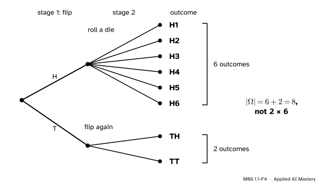
List the branches. The tree has two stages.
M06.1.1-F4
The two-stage experiment as a tree. The second stage depends on the first, so the branches are counted by adding: six outcomes after heads, two after tails.
Count. After heads there are 6 outcomes and after tails there are 2, and no outcome is on both sides, so
\[
|\Omega| = 6 + 2 = 8 .
\]
The multiplication rule would give \({2 \times 6 = 12}\), which is wrong: it pretends that a die is rolled after tails as well. Adding branches always works; multiplying works only when every branch has the same number of choices.
Check the two rules. Every run of the experiment ends at one leaf of the tree (nothing is left out), and no run ends at two leaves (no overlaps). So this is a proper sample space. Note that its eight outcomes are not equally likely: H1 needs a head and then a 1, while TT needs two tails. Lesson M06.1.3 shows how to give outcomes probabilities that differ.
Code
First the finite sample spaces of the lesson, built with itertools.product, which forms every tuple with one entry from each list, like nested loops.
from itertools import productcoin = ["H", "T"]die = [1, 2, 3, 4, 5, 6]three_flips = ["".join(p) for p in product(coin, repeat=3)]two_dice =list(product(die, repeat=2)) # ordered pairs (first, second)print(three_flips)print(len(two_dice), "outcomes; the first five:", two_dice[:5])
The two-stage experiment of the worked example needs a loop, because the second stage depends on the first.
two_stage = []for first in coin:if first =="H": two_stage += [f"H{k}"for k in die] # heads: roll a dieelse: two_stage += [f"T{f}"for f in coin] # tails: flip againprint(two_stage, len(two_stage))sums =sorted({i + j for i, j in two_dice})unordered = {tuple(sorted(pair)) for pair in two_dice}print("sums:", len(sums), " unordered pairs:", len(unordered))
The coarser sample spaces are easy to compute from the ordered pairs, as the formal statement promised. For flips until the first head the list never ends, so a program can only produce it one outcome at a time: a generator. For the spinner there is no list at all; a program can only draw from it.
from itertools import count, isliceimport numpy as npdef flips_until_head():for n in count(1): # n = the flip on which the head arrivesyield"T"* (n -1) +"H"print(list(islice(flips_until_head(), 5)))rng = np.random.default_rng(0)print(rng.random(3)) # three spins, each a number in [0, 1)
This module’s interactive, the event explorer, lives in lesson M06.1.4. It draws the 36 outcomes of two dice as the grid you met here and lets you pick events on it, which is where the next lesson goes.
Pitfalls
M06.1.1-F5
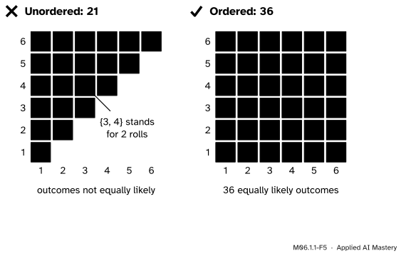
Wrong beside right. Forgetting the order squeezes two rolls, \({(3, 4)}\) and \({(4, 3)}\), into one item, while a double such as \({(2, 2)}\) stays a single roll. Keeping the order gives 36 outcomes of equal standing.
“With two dice, a 3 and a 4 is one outcome, so there are 21 outcomes.”
The 21 unordered pairs do form a sample space, but a lopsided one: the pair \({\{3, 4\}}\) happens in two ways and \({\{2, 2\}}\) in only one. Treat the 21 as equally likely and every answer is off. Imagine the dice painted different colours, keep the order, and use the 36 ordered pairs.
“Even, odd and less than 3 make a fine sample space for a die.”
Outcomes must not overlap. A roll of 2 is both even and less than 3, so it matches two items, and the list breaks the second rule. Items like these are events, sets of outcomes, which are the subject of the next lesson. The outcomes themselves are the six faces.
“The sample space of a classifier’s prediction is the labels it was trained on.”
List what can really come out. If the model can also return “not sure” when its confidence is low, that result belongs in \(\Omega\) too. A sample space that leaves out a possible result breaks the first rule. The probabilities given to the listed results are then made to add up to 1 without it, so taken together they are too large.
Check yourself
Recall
1. What is the sample space of an experiment?
Show answer
The set \(\Omega\) of all its possible outcomes, chosen so that each run of the experiment produces exactly one of them.
2. How many outcomes do three coin flips have, and why?
Show answer
Eight. Each flip has two results, so the multiplication rule gives \({2 \times 2 \times 2 = 8}\): HHH, HHT, HTH, HTT, THH, THT, TTH, TTT.
3. Why does the course record two dice as ordered pairs rather than as sums?
Show answer
The pair can answer every question about the roll, while the sum cannot say, for example, whether the first die shows a 6. For fair dice the 36 pairs are also equally likely; the 11 sums are not.
4. Give an example of a sample space that is countably infinite, and one that is continuous.
Show answer
Flips until the first head, \({\{H, TH, TTH, \dots\}}\), is countably infinite. The stopping point of a spinner, \({[0, 1)}\), is continuous.
5. When does the multiplication rule fail to count a sample space built in stages?
Show answer
When the choices at a later stage depend on what happened earlier. Then count the branches of the tree and add them.
Exercises
1.★ Write the sample space, and its size, for flipping a coin twice, and for rolling a die and then flipping a coin.
Show solution
Two flips: \({\Omega = \{HH, HT, TH, TT\}}\), so \({|\Omega| = 4}\). A die then a coin: outcomes are pairs such as \({(3, H)}\); \({\Omega = \{1, \dots, 6\} \times \{H, T\}}\) and \({|\Omega| = 6 \times 2 = 12}\).
2.★★ A classifier is run on three test emails, and each prediction is marked C (correct) or W (wrong). Write \(\Omega\) and its size. A colleague records only the number of correct predictions. Write that sample space, and give a question the first can answer but the second cannot.
Show solution
\(\Omega\) holds the eight strings CCC, CCW, CWC, CWW, WCC, WCW, WWC, WWW, so \({|\Omega| = 8}\), by the same tree as three coin flips. The colleague’s space is \({\{0, 1, 2, 3\}}\). “Was the first email predicted correctly?” is answered by any string (look at its first letter) but not by a count: a count of 2 could come from CCW or from WCC.
3.★★★ Roll a die until a 6 appears or three rolls have been made, whichever comes first. Record the rolls. How many outcomes are there?
Show solution
Sort the outcomes by how they end. A 6 on the first roll: one outcome, “6”. A first roll from 1 to 5, then a 6: five outcomes. Otherwise the first two rolls are not 6, giving \({5 \times 5 = 25}\) starts, and a third roll is always made, with 6 results, so \({25 \times 6 = 150}\) outcomes (25 of them end in a 6 and 125 do not). The stages depend on each other, so add the cases:
\[
|\Omega| = 1 + 5 + 150 = 156 .
\]
Summary card
List what could happen before asking how likely it is.
M06.1.1-F1
One experiment, 36 outcomes.
Sample space.\(\Omega\) is the set of all outcomes; each run gives exactly one.
Stages with fixed choices. Multiply: two dice have \({6 \times 6 = 36}\) outcomes.
Stages that depend on each other. Draw the tree and add the branches.
Three kinds. Finite, countably infinite (a list that never ends), continuous (no list).
Choose fine outcomes. A finer space can be made coarser, never the reverse.
Sources and next steps
Sources. Each was opened and checked against this lesson on 12 November 2026.
Jeremy Orloff and Jonathan Bloom, Reading 2: Probability, terminology and examples, MIT OpenCourseWare 18.05, Spring 2022. Section 2.1 defines experiment and sample space; Example 2 lists the eight outcomes of three tosses; Example 5 compares the 36 ordered pairs of two dice with the 11 sums, which are not equally likely; Section 2.3 calls finite and endless lists discrete and the interval from 0 to 1 continuous.
Charles M. Grinstead and J. Laurie Snell, Introduction to Probability, second edition (free PDF). Section 1.2: Definition 1.1 and the paragraph after it name the sample space \(\Omega\) and its elements, the outcomes; the same section treats countably infinite sample spaces, with the coin tossed until the first head (Example 1.13).
Python Software Foundation, itertools.product: the Cartesian product, like nested loops, with repeat pairing a list with itself.
Next.M06.1.2 Events as sets picks out groups of outcomes, such as “the sum is 7”, and combines them with or, and and not.