Typos on a page, requests in a second: many chances, each unlikely. Derive the Poisson PMF e^(-lambda) lambda^k / k! as the limit of Bin(n, lambda/n), show that it sums to 1 and that its mean and variance are both lambda, and set Bin(100, 0.03) beside Pois(3).
State the Poisson story and recognise counts that follow it.
Derive the Poisson PMF as the limit of Bin(n, lambda/n), factor by factor.
Show that the Poisson PMF sums to 1 and that its mean and variance are both lambda.
Compute Poisson probabilities by hand, by simulation and with scipy.stats.poisson, and judge when a Poisson can stand in for a binomial.
In review. The maths and code on this page are checked by automated tests on every change, but an independent reader has not signed it off yet. Spot a mistake or a confusing step? Tell us.
The question
A web service receives on average 3 requests per second. How often does a whole second pass with no request at all? How often do more than 6 arrive, enough to overload a small server? Counts like these are everywhere in machine learning: clicks on an advert, words in a document, defects on a production line. They have their own distribution, and it comes from the binomial.
From the last lesson
1. What does \({(1 + x/n)^n}\) tend to as \({n \to \infty}\)?
Show answer
\({e^x}\), for every real \(x\).
2. For \({T \sim \mathrm{Exp}(\lambda)}\), what is \({\Prob(T > t)}\)?
Show answer
\({e^{-\lambda t}}\).
Intuition
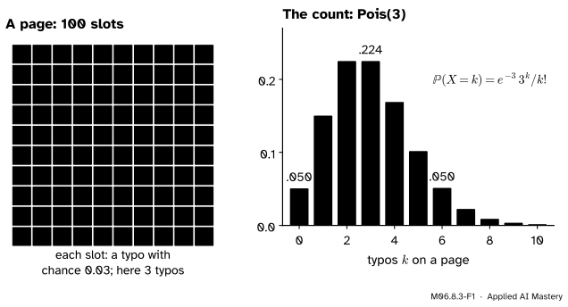
Think of a typed page with, on average, 3 typos. Each typo could sit in any of a great many places, and at each place a typo is unlikely. Cut the page into 100 slots, each holding a typo with chance 0.03. The number of typos is then a count of successes: \({\mathrm{Bin}(100, 0.03)}\).
M06.8.3-F1
Many chances, each unlikely. A page cut into 100 slots with a typo in each with chance 0.03 holds 3 typos on average; the count follows the Poisson bars on the right almost exactly.
But why 100 slots and not 1,000? The typos do not care how we cut the page. If we cut finer, each slot gets a smaller chance, \({3/n}\), so that the average stays 3. The Poisson distribution is what the count becomes when the cutting goes on for ever: it keeps only the average, \(\lambda\).
Build it up
Step 1. One window, \(n\) chances. Cut the window (a page, a second) into \(n\) slots, each holding an event with chance \({\lambda/n}\), independently. The count is \({X_n \sim \mathrm{Bin}(n, \lambda/n)}\), and its mean is \({n \cdot \lambda/n = \lambda}\) whatever \(n\) is.
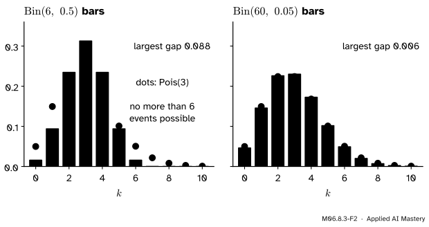
Step 2. Watch the bars settle. For \({\lambda = 3}\), compare \({n = 6}\) with \({n = 60}\).
M06.8.3-F2
\({\mathrm{Bin}(n, 3/n)}\) as bars and \({\mathrm{Pois}(3)}\) as dots. With 6 chances the bars cannot pass 6 and pile up in the middle; with 60 chances they lie almost on the dots.
Step 3. What survives. As \(n\) grows, \(n\) and \({p = \lambda/n}\) both drop out of the picture. Only their product \(\lambda\) remains. The formal statement takes the limit of the binomial PMF one factor at a time.
Step 4. The shape from one ratio. Once we have the formula \({p(k) = e^{-\lambda} \lambda^k / k!}\), dividing one bar by the bar before it cancels everything but one factor:
So the bars rise while \({k < \lambda}\), because each step multiplies by more than 1, and fall once \({k > \lambda}\). When \(\lambda\) is a whole number the two bars at \({\lambda - 1}\) and \(\lambda\) are equal: for \({\lambda = 3}\), the bars at 2 and 3 in the anchor figure both have height 0.224. The most likely count sits next to the mean, and the bars spread out on both sides, further to the right, since a count can grow without limit but cannot go below 0.
The formal statement
NoteDefinition: the Poisson distribution
\({X \sim \mathrm{Pois}(\lambda)}\), with \({\lambda > 0}\), when
It is the limit of \({\mathrm{Bin}(n, \lambda/n)}\) as \({n \to \infty}\), and its mean and its variance are both \(\lambda\).
In scipy.stats it is poisson(mu), with \({\mu = \lambda}\).
The limit, factor by factor. Fix \(k\). Write \({\binom{n}{k} = n(n - 1)\cdots(n - k + 1)/k!}\) and regroup the binomial PMF with \({p = \lambda/n}\) into four factors:
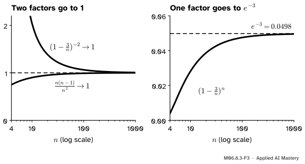
The first factor is a product of \(k\) fractions, \({\frac{n}{n} \cdot \frac{n-1}{n} \cdots}\), each of the form \({1 - j/n}\) with \({j < k}\). Each tends to 1, and there are a fixed number \(k\) of them, so their product tends to 1.
The second factor does not involve \(n\).
The third tends to \({e^{-\lambda}}\), by the limit \({(1 + x/n)^n \to e^x}\) of M06.8.2 with \({x = -\lambda}\).
The fourth is a fixed power of a number that tends to 1, so it tends to 1.
Multiplying the four limits gives \({e^{-\lambda} \lambda^k / k!}\).
M06.8.3-F3
The factors of the binomial chance of \({k = 2}\) events, with \({\lambda = 3}\), as \(n\) grows. Two tend to 1 and one tends to \({e^{-3}}\); what is left is the Poisson PMF.
It sums to 1. The Taylor series of the exponential, \({e^\lambda = \sum_{k \ge 0} \lambda^k/k!}\) (M04.8.4), gives
Its variance is \(\lambda\). The same trick on \({\E[X(X - 1)]}\), where the terms \({k = 0}\) and \({k = 1}\) are 0 and \({k(k - 1)/k! = 1/(k - 2)!}\):
So \({\E[X^2]} = {\E[X(X - 1)]} + {\E[X]} = {\lambda^2 + \lambda}\), and \({\mathrm{Var}(X)} = {\lambda^2 + \lambda - \lambda^2} = \lambda\). The binomial agrees in the limit: \({np(1 - p) = \lambda(1 - \lambda/n) \to \lambda}\).
A link to waiting. No event in a window of length \(t\) at rate \(\lambda\) per unit means a \({\mathrm{Pois}(\lambda t)}\) count of 0, with chance \({e^{-\lambda t}}\). That is exactly \({\Prob(T > t)}\) for the exponential wait of M06.8.2: the same slots, asked a different question.
Worked example
Requests arrive at 3 per second, so a second’s count is \({X \sim \mathrm{Pois}(3)}\). Find \({\Prob(X = 0)}\) and \({\Prob(X \le 2)}\), and compare with \({\mathrm{Bin}(100, 0.03)}\).
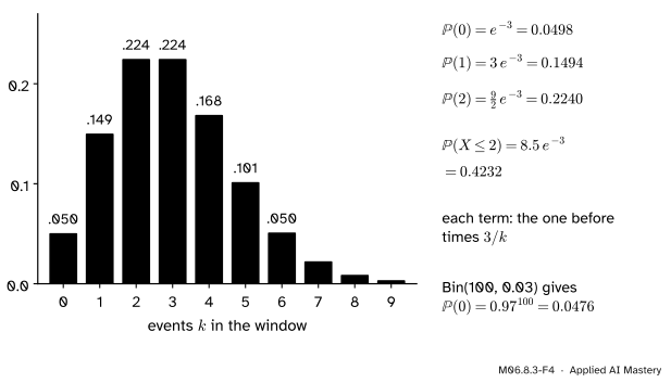
Bar by bar. Each bar is the one before times \({\lambda/k}\), because \({p(k) / p(k - 1) = \lambda/k}\):
About one second in twenty passes with no request. And by the complement, more than 6 requests arrive in \({1 - \Prob(X \le 6) = 0.0335}\) of seconds: about two seconds a minute.
M06.8.3-F4
The worked example as bars. The yellow bars are \({X \le 2}\); each bar is the one before times \({3/k}\), so the bars rise while \({k < 3}\) and fall after.
Beside the binomial. If a second really held 100 independent chances of 0.03, the count would be \({\mathrm{Bin}(100, 0.03)}\):
\(k\)
\({\mathrm{Bin}(100, 0.03)}\)
\({\mathrm{Pois}(3)}\)
0
0.0476
0.0498
1
0.1471
0.1494
2
0.2252
0.2240
3
0.2275
0.2240
4
0.1706
0.1680
The two agree to about two decimal places. The binomial needs \(n\) and \(p\); the Poisson needs only their product, which is often all we know.
A shorter window. In half a second the expected count is \({3 \times 0.5 = 1.5}\), so the count is \({\mathrm{Pois}(1.5)}\), and half a second with no request has chance \({e^{-1.5} = 0.2231}\). Seen from the other side, the wait for the next request is \({\mathrm{Exp}(3)}\) in seconds, and \({\Prob(T > 0.5) = e^{-3 \times 0.5}}\): the same number, as the link above promised.
Code
From scratch: the Poisson bars by the recurrence \({p(k) = p(k - 1) \cdot \lambda/k}\), and the binomial bars in exact fractions.
import mathfrom fractions import Fractiondef poisson_pmf(lam, kmax): bars = [math.exp(-lam)]for k inrange(1, kmax +1): bars.append(bars[-1] * lam / k) # each bar is the one before times lam / kreturn barspois = poisson_pmf(3, 60)p = Fraction(3, 100)binom = [math.comb(100, k) * p**k * (1- p) ** (100- k) for k inrange(101)]print("Pois(3): ", [round(q, 4) for q in pois[:5]], " P(X <= 2) =", round(sum(pois[:3]), 4))print("Bin(100,0.03):", [round(float(q), 4) for q in binom[:5]], " P(X <= 2) =", round(float(sum(binom[:3])), 4))mean =sum(k * q for k, q inenumerate(pois))var =sum(k * k * q for k, q inenumerate(pois)) - mean**2print("total", round(sum(pois), 12), " mean", round(mean, 10), " variance", round(var, 10)," P(X > 6) =", round(1-sum(pois[:7]), 4))
Simulation: 200,000 seconds as binomial counts and as Poisson counts.
import numpy as nprng = np.random.default_rng(seed=2)as_binomial = rng.binomial(n=100, p=0.03, size=200_000)as_poisson = rng.poisson(lam=3, size=200_000)for name, x in (("binomial", as_binomial), ("Poisson", as_poisson)):print(f"{name:9} share of 0: {(x ==0).mean():.4f} mean {x.mean():.3f} variance {x.var():.3f}")
binomial  share of 0: 0.0475  mean 3.002  variance 2.917
Poisson   share of 0: 0.0489  mean 3.004  variance 2.994
The Poisson counts have mean and variance both close to 3. The binomial counts have variance close to \({100 \times 0.03 \times 0.97 = 2.91}\), a little less. Last, SciPy, where the rate is called mu:
The module’s interactive, the distribution map, lives in lesson M06.8.4. Choose the arrow from binomial to Poisson, keep \({np = \lambda}\) fixed and step \(n\) up: the read-out gives the largest gap between the bars and the dots as it shrinks.
Pitfalls
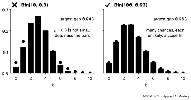
M06.8.3-F5
Wrong beside right. Both binomials have mean 3, but only the one with many unlikely chances is close to \({\mathrm{Pois}(3)}\).
“A binomial with mean 3 is close to Pois(3).”
Only when \(n\) is large and \(p\) is small. \({\mathrm{Bin}(10, 0.3)}\) has mean 3 but variance 2.1, and its bars miss the Poisson dots by up to 0.043. \({\mathrm{Bin}(100, 0.03)}\), with variance 2.91, is within 0.004.
“Any count is Poisson.”
The story needs events that happen independently and one at a time, at a steady rate. Requests that arrive in bursts, or clicks from a few heavy users, clump: their variance is far above their mean, while a Poisson count has variance equal to its mean. Compare the sample mean and variance of the counts before reaching for a Poisson.
“The rate is 3 per second, so a half-second window is Pois(3) too.”
The parameter is the expected count in the window you are counting. At 3 per second, a half-second window holds \({\mathrm{Pois}(1.5)}\), and a minute holds \({\mathrm{Pois}(180)}\).
Check yourself
Recall
1. What is the Poisson story?
Show answer
A count of events in a window, built from very many chances that are each unlikely and independent; only the expected count \(\lambda\) matters.
2. Which binomials does \({\mathrm{Pois}(\lambda)}\) approximate?
Show answer
\({\mathrm{Bin}(n, p)}\) with \(n\) large, \(p\) small and \({np = \lambda}\); it is the limit of \({\mathrm{Bin}(n, \lambda/n)}\).
3. Why does the Poisson PMF sum to 1?
Show answer
\({\sum_k \lambda^k / k! = e^{\lambda}}\), so the sum is \({e^{-\lambda} e^{\lambda} = 1}\).
4. What are the mean and the variance of \({\mathrm{Pois}(\lambda)}\)?
Show answer
Both are \(\lambda\).
5. For \({X \sim \mathrm{Pois}(3)}\), what is \({\Prob(X = 0)}\)?
Show answer
\({e^{-3} = 0.0498}\).
Exercises
1.★ A support desk receives on average 2 urgent tickets a day, as a Poisson count. Find the chance of a day with none, and of a day with at least one.
Show solution
\({\Prob(X = 0) = e^{-2} = 0.1353}\), and by the complement \({\Prob(X \ge 1) = 1 - e^{-2} = 0.8647}\).
2.★★ Each of 500 images in a data set is mislabelled with chance 0.004, independently. Find the exact chance that none is mislabelled, and its Poisson approximation.
Show solution
Exactly, the count is \({\mathrm{Bin}(500, 0.004)}\) and \({\Prob(X = 0) = 0.996^{500} = 0.1348}\). With \({\lambda = 500 \times 0.004 = 2}\), the Poisson gives \({e^{-2} = 0.1353}\). The two differ by 0.0005: many chances, each unlikely.
3.★★★ Let \({X \sim \mathrm{Pois}(a)}\) and \({Y \sim \mathrm{Pois}(b)}\) be independent. Show that \({X + Y \sim \mathrm{Pois}(a + b)}\).
Show solution
Add the products along a diagonal (M06.5.4): \({X + Y = n}\) when \({X = k}\) and \({Y = n - k}\) for some \({k = 0, \ldots, n}\). So
using \({n!/(k!\,(n - k)!) = \binom{n}{k}}\) and then the binomial theorem. In the story: requests counted in two separate windows add up to the requests in the combined window.
Summary card
Many chances, each unlikely: the count is Poisson, and only its mean λ matters.
M06.8.3-F1
A count of rare events.
PMF.\({e^{-\lambda} \lambda^k / k!}\) for \({k = 0, 1, 2, \ldots}\); each bar is the one before times \({\lambda/k}\).
Sources. Each was opened and checked against this lesson on 12 November 2026.
Hossein Pishro-Nik, Introduction to Probability, Statistics, and Random Processes, Section 3.1.5: the Poisson PMF, its story of counts in an interval, and the theorem in “Poisson as an approximation for binomial” that \({\mathrm{Bin}(n, \lambda/n)}\) tends to \({\mathrm{Pois}(\lambda)}\). Section 3.2.2 finds the Poisson mean \(\lambda\) with the series for \({e^\lambda}\).
Chris Piech, Probability for Computer Scientists, Poisson Distribution: a window cut into \(n\) buckets with \({p = \lambda/n}\), the limits \({(1 - \lambda/n)^n \to e^{-\lambda}}\) and \({n!/(n - x)! \to n^x}\), mean and variance \(\lambda\), and changing the window by scaling the rate.
SciPy developers, scipy.stats.poisson (SciPy 1.18 reference): PMF \({\exp(-\mu)\, \mu^k / k!}\) for \({k \ge 0}\), with shape parameter mu.
Next.M06.8.4 A map of the families puts every family met so far on one map. Events spread through time, the Poisson process, return in M07.8, and Poisson regression, which models a count whose rate depends on inputs, in S03.8.