import math
import numpy as np
import torch
from torch import nn
from torch.utils.data import DataLoader, TensorDataset
from sklearn.datasets import make_moons
from sklearn.model_selection import train_test_split

torch.set_num_threads(1)
X, labels = make_moons(n_samples=200, noise=0.2, random_state=0)
X_train, X_val, y_train, y_val = train_test_split(X, labels, test_size=0.25,
                                                  stratify=labels, random_state=0)
X_train, X_val = torch.tensor(X_train, dtype=torch.float32), torch.tensor(X_val, dtype=torch.float32)
y_train, y_val = torch.tensor(y_train), torch.tensor(y_val)
loss_fn = nn.CrossEntropyLoss()

def make_model(width=16, seed=0):
    torch.manual_seed(seed)
    return nn.Sequential(nn.Linear(2, width), nn.ReLU(), nn.Linear(width, width), nn.ReLU(),
                         nn.Linear(width, 2))

def loader(X, y, batch_size=32, shuffle=True):
    return DataLoader(TensorDataset(X, y), batch_size=batch_size, shuffle=shuffle,
                      generator=torch.Generator().manual_seed(0))

def train_one_epoch(model, loss_fn, optimizer, data):
    model.train()
    total, count = 0.0, 0
    for X, y in data:
        loss = loss_fn(model(X), y)
        optimizer.zero_grad()
        loss.backward()
        optimizer.step()
        total += loss.item() * len(y)
        count += len(y)
    return total / count

def evaluate(model, loss_fn, data):
    model.eval()
    total, count = 0.0, 0
    with torch.no_grad():
        for X, y in data:
            total += loss_fn(model(X), y).item() * len(y)
            count += len(y)
return total / countFirst checks when training fails
Three quick checks catch most broken training loops before any tuning: a starting loss near ln K, one small batch learned by heart, and a learning rate whose loss falls. Then read the curves: no progress, divergence and a widening gap.
Before this lesson: DL01.8.2 Epochs, validation and the two modes
What you will be able to do
- Derive why the starting loss of a K-class classifier with small logits is close to ln K, and use it as a check.
- Run the one-batch overfitting check and explain what its failure says about the loop.
- Recognise a learning rate that is too small or too large from the loss curve, including a loss that becomes NaN.
- Read training and validation curves for no progress, divergence and a widening gap.
The question
You start a training run and the loss does not go down, or goes down and then up, or prints nan. The bug could be in the data, the model, the loss, the five lines or the learning rate, and a network gives no error message for any of them. Which few checks, each taking seconds, tell you where to look before you start changing anything?
From the last lesson
1. Write the epoch loss in terms of the batch means \(L_k\) and the batch sizes \(\abs{B_k}\).
Show answer
\({\bar L = \frac1n \sum_k \abs{B_k} L_k}\), the mean loss over all \(n\) examples.
2. What does model.eval() change, and what does torch.no_grad() change?
Show answer
eval() switches layers such as dropout and normalisation to their testing behaviour. no_grad() stops the graph from being recorded. They are independent.
Intuition
A training loop has many parts and fails quietly. The fastest way to find a broken part is to test the whole loop against numbers you can predict before it runs. Three such numbers exist, and they come in a natural order: one before training starts, one on a tiny problem, one on the real run.
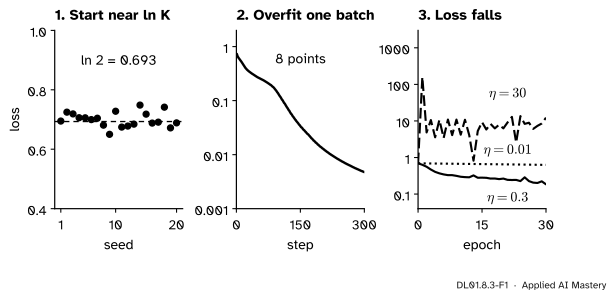
The three checks on the make_moons network of this module, each with the number to expect: a starting loss near ln 2, a loss near zero on one small batch, and a loss that falls.
- Start near ln K. Before any update, a network that has learned nothing should be equally unsure of every class, so its loss should be close to the loss of guessing uniformly.
- Overfit one batch. A network with hundreds of parameters can learn eight points by heart. If the loss on them will not go to nearly zero, the loop is broken, whatever the learning rate.
- Make the loss fall. On the real data, the loss should fall steadily. A loss that crawls means the steps are too small; one that rises or turns into
nanmeans they are too large.
Build it up
Check 1, the number. The cross-entropy of one example is \({-\ln p_y}\), minus the log of the probability given to its true class (DL01.4.3). If the network gives every class the same probability \({1/K}\), every example costs \({-\ln(1/K) = \ln K}\). For two classes that is \({\ln 2 \approx 0.693}\), for the ten digits of DL01.10 \({\ln 10 \approx 2.303}\).
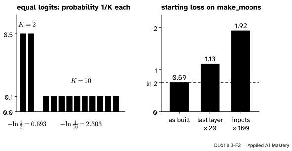
Left: equal logits give the probability \({1/K}\) to each class and the loss \({\ln K}\). Right: the network as built starts at ln 2; two broken set-ups start far above it.
A starting loss well above ln K means the network is confidently wrong before it has learned anything. The right-hand panel shows two common causes. Inputs that were never scaled (here multiplied by 100, as if measured in centimetres instead of metres) make the logits huge. A last layer with large weights does the same. Both waste the first part of training on undoing the overconfidence, and both are easy to fix once the number has flagged them.
Check 2, the reason. The 2-16-16-2 network has 354 parameters; eight points give it eight constraints. Driving their loss towards zero needs only a working forward pass, a correct loss, a backward pass that reaches every parameter and an optimizer that moves them. If it fails, one of those four is broken: no amount of tuning will help.
Check 3, the reading. Try a few learning rates spaced by factors of about 10 to 100 and watch the first epochs. The healthy one falls quickly at first and then more slowly.
The formal statement
Derivation. Take \({K}\) out of the sum:
\[ \begin{aligned} \ln \sum_j e^{z_j} &= \ln\Big(K \cdot \frac1K \sum_j e^{z_j}\Big) \\ &= \ln K + \ln\Big(\frac1K \sum_j e^{z_j}\Big). \end{aligned} \]
For small \(z_j\), \({e^{z_j} \approx 1 + z_j}\), so the mean inside the last logarithm is about \({1 + \bar z}\), and \({\ln(1 + \bar z) \approx \bar z}\). Hence \({\ln \sum_j e^{z_j} \approx \ln K + \bar z}\), and subtracting \(z_y\) gives the result. If every logit is the same, the mean of the \(e^{z_j}\) is exactly \(e^{\bar z}\), its logarithm is exactly \(\bar z = z_y\), and \({\ell = \ln K}\).
A network that has not been trained has no reason to favour the true class, so \({z_y - \bar z}\) is as often positive as negative and roughly cancels in the mean over many examples. Its starting loss is therefore near ln K. PyTorch’s default start gives small logits for inputs of size about 1, which is why the moons network starts at about 0.695.
Why ln K is the right bar. For balanced classes, ln K is also the best a model can do that ignores the input and always predicts the same probabilities \(q\): the mean loss of such a model is the cross-entropy between the class proportions (all \(1/K\)) and \(q\), which is the entropy ln K plus a Kullback-Leibler divergence that is never negative and is zero only for \({q}\) uniform (DL01.4.3). A trained network that cannot beat ln K has learned nothing from the inputs.
Why large steps diverge, and how NaN appears. Near a minimum the loss is roughly a parabola with curvature \(h\) along its steepest direction. ML01.5.3 showed that gradient descent shrinks the error by the factor \({(1 - \eta h)}\) per step, so it converges only for \({\eta < 2/h}\) and grows beyond. Once the loss is large, the logits are large, and in 32-bit floating point a number above about \({3.4 \times 10^{38}}\) becomes inf; then inf - inf gives nan, and one nan in a gradient spreads to every weight after the next step.
Worked example
Check 1 by hand. Four examples of a two-class network have small logits: \({(0.2, 0.0)}\) with label 0, \({(0.1, 0.1)}\) with label 1, \({(-0.1, 0.2)}\) with label 0 and \({(0.0, 0.3)}\) with label 1. For two classes the cross-entropy depends only on the margin \({d = z_y - z_{\text{other}}}\):
\[ \begin{aligned} \ell &= -z_y + \ln(e^{z_y} + e^{z_{\text{other}}}) \\ &= \ln(1 + e^{-d}). \end{aligned} \]
The margins are \({0.2}\), \({0}\), \({-0.3}\) and \({0.3}\). The losses are \({\ln(1 + e^{-0.2}) \approx 0.598}\), \({\ln 2 \approx 0.693}\), \({\ln(1 + e^{0.3}) \approx 0.854}\) and \({\ln(1 + e^{-0.3}) \approx 0.554}\). Their mean is \({2.700/4 \approx 0.675}\).
The formal statement predicts this. For two classes, \({z_y - \bar z = d/2}\), and the next term of the expansion of \({\ln(1 + e^{-d})}\) about 0 is \({d^2/8}\), so the mean loss is about
\[ \begin{aligned} &\ln 2 - \tfrac12 \bar d + \tfrac18 \overline{d^2} \\ &\quad= 0.693 - 0.025 + 0.007 = 0.675, \end{aligned} \]
with \({\bar d = 0.05}\) the mean margin and \({\overline{d^2} = 0.055}\) the mean squared margin. The check passes: 0.675 is close to 0.693.
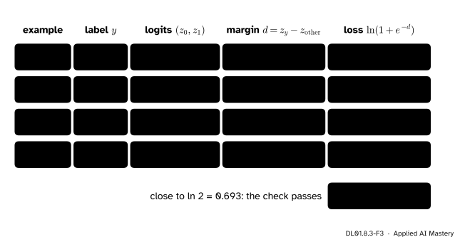
Check 1 traced by hand. Small logits give losses scattered around ln 2, and their mean lands close to it.
Check 1 failing. Multiply the same logits by 30, as unscaled inputs might. The margins become 6, 0, \(-9\) and 9, with losses about 0.0025, 0.693, 9.0001 and 0.0001, whose mean is about 2.42: far above ln 2, and dominated by one confidently wrong example.
Code
The module’s data and network, and the evaluate function of DL01.8.2.
Check 1: the starting loss.
def check_start(model, loss_fn, data, K):
    loss = evaluate(model, loss_fn, data)
    return loss, math.log(K)

train_data = loader(X_train, y_train, shuffle=False)
start, target = check_start(make_model(), loss_fn, train_data, K=2)
starts = [check_start(make_model(seed=s), loss_fn, train_data, K=2)[0] for s in range(20)]
scaled = check_start(make_model(), loss_fn, loader(100 * X_train, y_train, shuffle=False), K=2)[0]
print(f"as built {start:.3f} against ln 2 = {target:.3f}; twenty seeds: {min(starts):.2f} to {max(starts):.2f}")
print(f"inputs times 100: {scaled:.2f}")

d = np.array([0.2, 0.0, -0.3, 0.3])
print("worked example:", np.round(np.log1p(np.exp(-d)), 3), round(float(np.log1p(np.exp(-d)).mean()), 3),
      " logits times 30:", round(float(np.log1p(np.exp(-30 * d)).mean()), 2))
as built 0.695 against ln 2 = 0.693; twenty seeds: 0.65 to 0.75
inputs times 100: 1.92
worked example: [0.598 0.693 0.854 0.554] 0.675 logits times 30: 2.42Check 2: overfit one batch. Eight training points, 300 steps. Then the same with a classic wiring bug: the model is rebuilt after the optimizer was created, so the optimizer updates the parameters of a model that is no longer used.
def overfit_one_batch(model, optimizer, X, y, steps=300):
    model.train()
    for _ in range(steps):
        loss = loss_fn(model(X), y)
        optimizer.zero_grad()
        loss.backward()
        optimizer.step()
    return loss.item()

xb, yb = X_train[:8], y_train[:8]
model = make_model()
healthy = overfit_one_batch(model, torch.optim.SGD(model.parameters(), lr=0.3), xb, yb)

stale_optimizer = torch.optim.SGD(make_model().parameters(), lr=0.3)
model = make_model()                     # the bug: a new model, but the old optimizer
broken = overfit_one_batch(model, stale_optimizer, xb, yb)
print(f"one batch, healthy loop: {healthy:.4f}   wiring bug: {broken:.4f}")
one batch, healthy loop: 0.0047 wiring bug: 0.7327Check 3: three learning rates, and one more to show nan.
def lr_check(lrs, epochs=30):
    results = {}
    for lr in lrs:
        model = make_model()
        optimizer = torch.optim.SGD(model.parameters(), lr=lr)
        data = loader(X_train, y_train)
        losses = [train_one_epoch(model, loss_fn, optimizer, data) for _ in range(epochs)]
        results[lr] = (losses[0], losses[-1], math.isfinite(losses[-1]))
    return results

for lr, (first, last, finite) in lr_check([0.01, 0.3, 30, 3000]).items():
    print(f"lr {lr:>6}: epoch 1 {first:12.4g}   epoch 30 {last:8.4g}   finite: {finite}")
lr 0.01: epoch 1 0.6938 epoch 30 0.6298 finite: True
lr 0.3: epoch 1 0.6706 epoch 30 0.1991 finite: True
lr 30: epoch 1 1.241e+05 epoch 30 6.864 finite: True
lr 3000: epoch 1 4.118e+30 epoch 30 nan finite: FalseAt 0.01 the loss has barely left ln 2 after 30 epochs. At 0.3 it falls to about 0.2. At 30 the first epoch averages above \(10^4\) and the loss never comes back below its start. At 3000 it overflows to nan.
Reading the curves: a widening gap. A wider 2-64-64-2 network on only 30 of the training points, in batches of 10, is free to memorise them.
model = make_model(width=64)
optimizer = torch.optim.SGD(model.parameters(), lr=0.5)
small = loader(X_train[:30], y_train[:30], batch_size=10)
history = {"train": [], "val": []}
for epoch in range(150):
    train_one_epoch(model, loss_fn, optimizer, small)
    history["train"].append(evaluate(model, loss_fn, loader(X_train[:30], y_train[:30], shuffle=False)))
    history["val"].append(evaluate(model, loss_fn, loader(X_val, y_val, shuffle=False)))

best = int(np.argmin(history["val"])) + 1
print(f"validation lowest at epoch {best}: {min(history['val']):.3f};  "
      f"at epoch 150: training {history['train'][-1]:.4f}, validation {history['val'][-1]:.3f}")
validation lowest at epoch 73: 0.079; at epoch 150: training 0.0045, validation 0.241The training loss heads for zero while the validation loss, after reaching its lowest value, climbs to about three times that. That is overfitting (ML01.8): the network fits the 30 points better and the rest of the moons worse. The exact epochs depend on floating-point details of the machine; the shape does not.
Explore
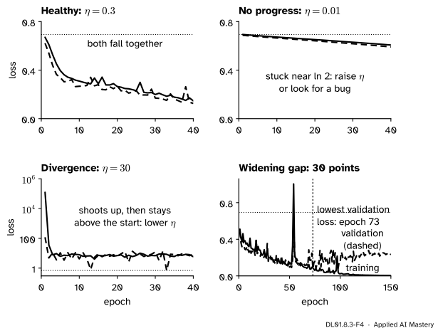
Four shapes of the curves and what they say: healthy, no progress, divergence and a widening gap.
Each shape points at a different fix. No progress near ln K: raise the learning rate, and if that does not help, go back to check 2. Divergence: lower the learning rate. A widening gap: the weights at the bottom of the validation curve are the ones to keep, which DL01.8.4 does automatically; more data and the regularisation of DL02.5 shrink the gap itself. The loop stepper in DL01.8.1 has a learning-rate slider: push it up until the loss curve starts to jump.
Pitfalls
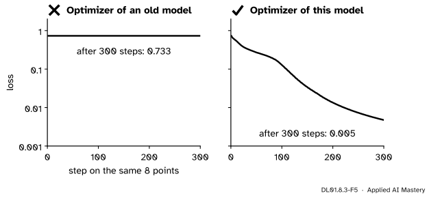
Wrong beside right. With an optimizer that holds another model’s parameters, nothing is learned and no error is raised. Check 2 exposes it in seconds.
“The loss is not falling, so the learning rate must be wrong.”
Maybe, but first run check 2. In the figure no learning rate would help: the optimizer updates parameters that the model no longer uses. Detached tensors, a forgotten step, or a loss computed on the wrong outputs fail the same way.
“A starting loss of 1.9 instead of 0.69 is just a bad start; training will fix it.”
Often it does, slowly, but it is a symptom: inputs on the wrong scale or an overconfident last layer. The same bug can hide in the test data, where training cannot fix it. Find the cause.
“The validation loss is rising, so the run is broken: stop and start again.”
If the training loss is still falling, this is overfitting, not a bug. The run already passed through the best weights it will find. Keep them (DL01.8.4) rather than throwing the run away.
Check yourself
Recall
1. What starting loss should a classifier with 2 classes, and one with 10, show, and why?
Show answer
About \({\ln 2 \approx 0.693}\) and \({\ln 10 \approx 2.303}\). With small logits every class gets probability about \(1/K\), and \({-\ln(1/K) = \ln K}\).
2. What does it mean if a network cannot drive the loss on eight training points close to zero?
Show answer
The loop is broken: the forward pass, the loss, the backward pass or the optimizer’s link to the parameters. Tuning will not fix it.
3. Write the two-class cross-entropy in terms of the margin \(d\).
Show answer
\({\ell = \ln(1 + e^{-d})}\) with \({d = z_y - z_{\text{other}}}\).
4. Name two signs that the learning rate is too large.
Show answer
The loss rises (often jumping far above its start in the first epoch) or becomes nan.
5. Training loss falling, validation loss rising: what is it, and which weights do you want?
Show answer
Overfitting. The weights from the epoch with the lowest validation loss.
Exercises
1. ★ A ten-class digit classifier starts at a loss of 2.31; another starts at 9.5. Which one passes check 1, and what could be wrong with the other?
Show solution
\({\ln 10 \approx 2.303}\), so the first passes. The second is far above: its logits are large before any training, so it is confidently wrong. Likely causes are pixels left on the scale 0 to 16 instead of being divided by 16, or a last layer with large weights.
2. ★★ Three classes have logits \({(0.1, -0.2, 0.1)}\), and the true class is the middle one, with logit \(-0.2\). Compute the exact loss and the approximation \({\ln 3 - (z_y - \bar z)}\).
Show solution
The mean logit is \({\bar z = (0.1 - 0.2 + 0.1)/3 = 0}\), so the approximation is
\[ \begin{aligned} \ln 3 - (-0.2 - 0) &= 1.0986 + 0.2 \\ &= 1.2986 . \end{aligned} \]
Exactly, \({\ell = 0.2 + \ln(e^{0.1} + e^{-0.2} + e^{0.1})}\). The three exponentials are 1.10517, 0.81873 and 1.10517, with sum 3.02907 and logarithm 1.10826, so \({\ell \approx 1.3083}\). The approximation is off by 0.01, the size of the squared terms it drops.
3. ★★★ Show that for two classes \({z_y - \bar z = d/2}\), and use the expansion \({\ln(1 + e^{-d}) \approx \ln 2 - d/2 + d^2/8}\) to explain why the starting loss of a network with random small logits tends to sit slightly above ln 2 on average.
Show solution
With two logits, \({\bar z = (z_y + z_{\text{other}})/2}\), so \({z_y - \bar z = (z_y - z_{\text{other}})/2 = d/2}\). For the expansion, let \({f(d) = \ln(1 + e^{-d})}\). Then \({f(0) = \ln 2}\), \({f'(d) = -e^{-d}/(1 + e^{-d})}\) with \({f'(0) = -\tfrac12}\), and \({f''(d) = e^{-d}/(1 + e^{-d})^2}\) with \({f''(0) = \tfrac14}\), which gives \({\ln 2 - d/2 + d^2/8}\). If the margins of an untrained network are as often positive as negative, the mean of \(d\) is about 0 but the mean of \(d^2\) is positive, so the mean loss is about \({\ln 2 + \overline{d^2}/8}\): slightly above ln 2. The twenty seeds in the figure scatter between 0.65 and 0.75 because on 150 points the mean margin is not exactly zero.
Summary card
Before tuning: start near ln K, overfit one batch, make the loss fall.
Three numbers to predict before training.
- Starting loss: \({\ell \approx \ln K - (z_y - \bar z)}\), about ln K (0.693 for 2 classes, 2.303 for 10).
- One small batch: loss to nearly zero, or the loop is broken.
- Learning rate: crawling means too small; rising or
nanmeans too large. - Curves: flat near ln K, divergence, or a widening gap each have their own fix.
Sources and next steps
Sources. Each was opened and checked against this lesson on 15 November 2026.
- Stanford CS231n, Neural Networks Part 3: Learning and Evaluation. Under sanity checks: “look for correct loss at chance performance”, with an expected initial loss of 2.302 for ten classes, and “overfit a tiny subset of data”, called the most important check. Under babysitting the learning process: how the loss curve looks for low, high and good learning rates, and the gap between training and validation accuracy as a measure of overfitting.
- Andrej Karpathy, A Recipe for Training Neural Networks (2019), step 2: “verify loss @ init”, with \({-\log(1/n_{\text{classes}})}\) for a softmax, and “overfit one batch” of as few as two examples.
- PyTorch 2.15 documentation,
torch.nn.CrossEntropyLoss: takes unnormalised logits and integer class labels, and withreduction='mean'averages the per-example losses \({-\ln\big(e^{z_{y}} / \sum_c e^{z_c}\big)}\).
Next. DL01.8.4 Checkpoints and a reusable fit function keeps the best weights of a run automatically and makes a run repeatable and resumable.
This lesson unlocks
DL01.8.4 Checkpoints and a reusable fit function
Your progress is saved in this browser only. No account, no tracking.