nn.Linear stores its weight with shape (out, in) and computes x W-transpose + b, exactly as the course does. Build networks with nn.Sequential and your own Module, count and name their parameters, read a state_dict, and copy NumPy weights in to get the same outputs.
DL01.7.3L2 Intermediate25 minIn review (what this means)
The maths and code on this page are checked by automated tests on every change, but an independent reader has not signed it off yet. Spot a mistake or a confusing step? Tell us.
Explain what nn.Linear stores and computes, with the shapes of its weight, its bias, its input and its output.
Build a network with nn.Sequential and with a custom nn.Module that defines forward.
List and count a network’s parameters with parameters() and named_parameters(), and check the count against the sum of n_l (n_(l-1) + 1).
Read and load a state_dict, and copy NumPy weights into a module so that it gives the same outputs.
The question
Your DL01.6 library had a Parameter, a Module with parameters(), a Linear with weight of shape (out, in), and a Sequential. PyTorch’s torch.nn uses the same names on purpose. Copy the weights of a 2-16-16-2 network from NumPy into PyTorch’s version: does it give the same outputs, and how do you even find the 354 numbers inside it?
From the last lesson
1. Which tensors receive a .grad when you call L.backward()?
Show answer
The leaves with requires_grad=True, such as the weights and biases; intermediate results do not.
2. What happens to .grad if you run forward and backward twice without clearing it?
Show answer
The second gradient is added to the first, so .grad holds their sum.
Intuition
A module is an object that holds parameters and knows how to compute with them. Modules nest: a network is a module whose parts are modules. Whenever you assign a module or an nn.Parameter as an attribute of a module, it is registered, so the outer module can find it, and so can every tool that asks the outer module for its parameters.
DL01.7.3-F1
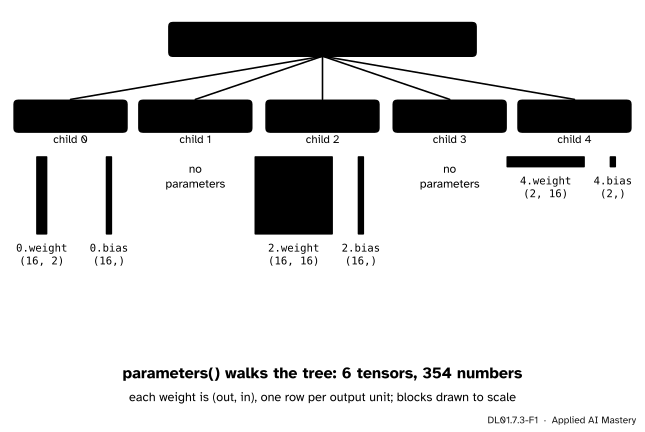
A network is a tree of modules. Only the Linear layers own parameters, each a weight of shape (out, in) and a bias. named_parameters() walks the tree and names each one by its path: 0.weight is the weight of child 0.
The tree is what makes the rest easy. To count the network’s numbers, walk the tree. To save the network, walk the tree and store every tensor under its name. To hand the weights to an optimizer, walk the tree and pass the list. Your DL01.6.3 Module.parameters() did the first of these by recursion; torch.nn.Module does all three.
Build it up
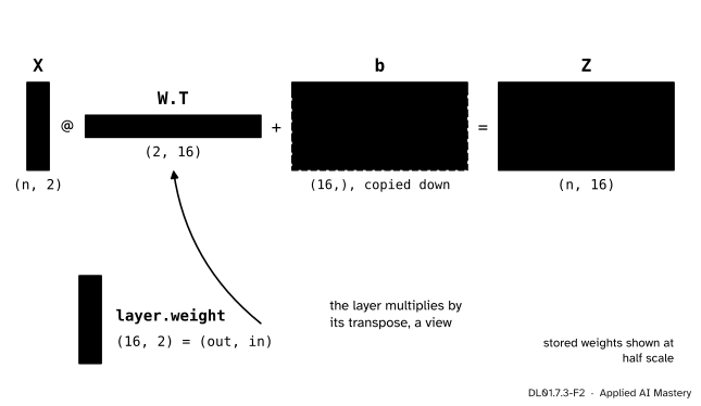
Step 1. One layer.nn.Linear(2, 16) creates a weight of shape \((16, 2)\) and a bias of shape \((16,)\), both nn.Parameters, that is tensors with requires_grad=True. Called on a batch \(\mat{X}\) with rows as examples, it returns \(\mat{X}\mat{W}\T + \vect{b}\): the course’s convention, so no transpose has to be remembered when weights move between NumPy and PyTorch.
DL01.7.3-F2
What nn.Linear(2, 16) stores and computes. The weight is kept as (out, in), one row per output unit; the layer multiplies by its transpose and broadcasts the bias down the batch.
Step 2. A chain.nn.Sequential(nn.Linear(2, 16), nn.ReLU(), nn.Linear(16, 16), nn.ReLU(), nn.Linear(16, 2)) calls its children in order, each on the output of the one before. Its children are numbered from 0, and the activations count as children even though they hold nothing.
Step 3. Your own module. Subclass nn.Module, call super().__init__() first, assign the layers as attributes in __init__, and write forward. Calling the module, model(X), runs forward (with some bookkeeping around it); do not call forward directly.
Step 4. Finding the parameters.model.parameters() yields every registered parameter, of this module and of every submodule. model.named_parameters() yields (name, tensor) pairs. Counting is one line: sum(p.numel() for p in model.parameters()).
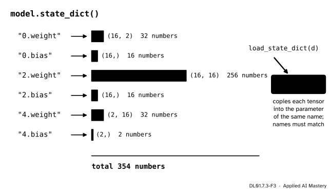
Step 5. The state.model.state_dict() is an ordered dictionary from each name to its tensor, detached from the graph but sharing memory with the parameter. model.load_state_dict(d) copies the tensors of d into the module’s own parameters, and by default insists that the names match exactly.
The formal statement
What a linear layer computes. For nn.Linear(n_in, n_out) with weight \(\mat{W}\) of shape \((n_\text{out}, n_\text{in})\) and bias \(\vect{b}\) in \(\R^{n_\text{out}}\), an input \(\mat{X}\) of shape \((n, n_\text{in})\) gives
of shape \((n, n_\text{out})\). Row \(i\) of \(\mat{Z}\) is \(\mat{W}\vect{x}_i + \vect{b}\), the column form of DL01.1.3 written as a row. Leading axes beyond the batch are allowed: any input of shape \((\ldots, n_\text{in})\) gives \((\ldots, n_\text{out})\).
How many parameters. A multilayer perceptron with widths \(n_0, n_1, \dots, n_D\) has, in layer \(l\), a weight of \(n_l \times n_{l-1}\) numbers and a bias of \(n_l\), so
How it starts. A new nn.Linear draws every weight and every bias independently from the uniform distribution on \({[-1/\sqrt{n_\text{in}},\; 1/\sqrt{n_\text{in}}]}\). Why this range, and what better choices exist, is the subject of DL02.3; here it only matters that two networks built from the same seed start from the same numbers.
DL01.7.3-F3
A state_dict is a dictionary from names to tensors: the whole network as data. Saving a network (DL01.8.4) is saving this dictionary, and loading copies it back into a network of the same shape.
Go deeper: why a module finds its parameters without being told
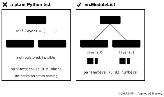
nn.Module overrides attribute assignment. When __init__ runs self.fc1 = nn.Linear(2, 16), the module notices that the value is a Module and stores it in an internal ordered dictionary of children, self._modules, under the name fc1; an nn.Parameter goes into self._parameters. named_parameters() then walks these dictionaries recursively, joining names with dots. That is also why super().__init__() must come first: it creates those dictionaries. A Python list of layers is an ordinary value, so its layers are not registered, which the pitfalls below show; nn.ModuleList is the registered version of a list.
Worked example
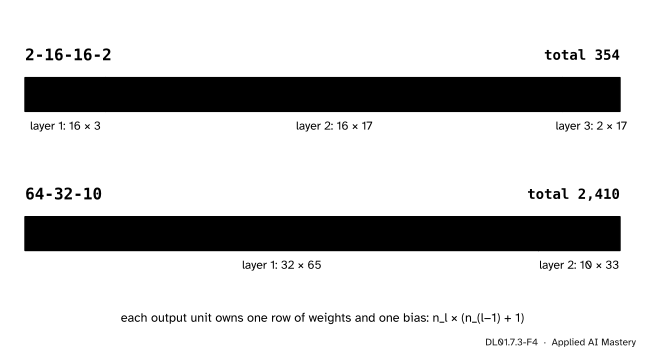
Count the 2-16-16-2 network. Layer 1 maps 2 inputs to 16 units: \({16 \cdot (2 + 1)} = 48\). Layer 2 maps 16 to 16: \({16 \cdot (16 + 1)} = 272\). Layer 3 maps 16 to 2: \({2 \cdot (16 + 1)} = 34\). The total is \(48 + 272 + 34 = 354\).
Count the 64-32-10 network that DL01.10 trains on the digit images. Layer 1: \({32 \cdot (64 + 1)} = 2{,}080\). Layer 2: \({10 \cdot (32 + 1)} = 330\). The total is \(2{,}410\).
DL01.7.3-F4
The parameter count, layer by layer. Each output unit owns one row of weights and one bias, so a layer holds \({n_l (n_{l-1} + 1)}\) numbers. The square middle layer dominates the small network; the first layer dominates the digit network.
Read one name. In the Sequential, the second Linear is child 2 (child 1 is the ReLU), so its weight is called 2.weight, with shape \((16, 16)\). In a custom module with self.hidden2 = nn.Linear(16, 16), the same tensor is called hidden2.weight. The names follow the attributes, so two networks with the same layers but different attribute names cannot load each other’s state_dict without renaming.
Code
One layer first, checked against the formula and the initial range.
Now the copy. The engine of DL01.6 keeps each weight as a NumPy array of shape (out, in) inside its Tensor, and DL01.6.4 starts its 2-16-16-2 network from the weights of DL01.5.4: normal draws with standard deviation \(\sqrt{2/n_\text{in}}\) from np.random.default_rng(0), and zero biases. We draw the same arrays here. The NumPy forward pass is the one of DL01.7.1 with a linear output, run on the 200 points of make_moons.
rng = np.random.default_rng(0) # the generator of DL01.5.4 and DL01.6.4sizes = [2, 16, 16, 2]weights = [(rng.normal(0, np.sqrt(2/ k), (m, k)), np.zeros(m)) for k, m inzip(sizes[:-1], sizes[1:])]def forward_np(X, params): A = Xfor l, (W, b) inenumerate(params): Z = A @ W.T + b A = np.maximum(Z, 0.0) if l <len(params) -1else Zreturn AX, y = make_moons(n_samples=200, noise=0.2, random_state=0)model = nn.Sequential(nn.Linear(2, 16), nn.ReLU(), nn.Linear(16, 16), nn.ReLU(), nn.Linear(16, 2)).double()state = {}for index, (W, b) inzip([0, 2, 4], weights): state[f"{index}.weight"] = torch.from_numpy(W) state[f"{index}.bias"] = torch.from_numpy(b)print(model.load_state_dict(state))with torch.no_grad(): out_torch = model(torch.from_numpy(X))out_np = forward_np(X, weights)gap = (out_torch - torch.from_numpy(out_np)).abs().max().item()print(tuple(out_torch.shape), f"largest difference {gap:.1e}")
<All keys matched successfully>
(200, 2) largest difference 0.0e+00
The outputs agree to rounding: the largest difference is at most a few units in the last bit of a float64, about \(10^{-16}\), and on some machines it is exactly 0. Bit for bit equality is not promised, because the two libraries may add the products of a matrix row in a different order, and floating-point addition is not associative. load_state_dict copied the numbers, so changing the NumPy arrays afterwards does not reach the module, while the state_dict it returns shares memory with the module’s parameters.
Explore
This module’s interactive, Shapes and strides, lives in DL01.7.1. Here, try the code: give MLP a fourth layer, predict the new count from \(\sum_l {n_l (n_{l-1} + 1)}\), and check it with count.
Pitfalls
DL01.7.3-F5
Wrong beside right. Layers kept in a Python list are invisible to the module: it reports no parameters, and an optimizer given model.parameters() trains nothing. nn.ModuleList registers them.
“I put my layers in a list, so they are part of the model.”
A Python list is not a module, so nn.Module does not look inside it. parameters() misses those layers, state_dict() does not save them, and .double() or .to(device) does not convert them. Use nn.ModuleList (or nn.Sequential) for a variable number of layers.
“The weights from scikit-learn will load as they are.”
scikit-learn’s coefs_, and the layer \(\mat{X}\mat{W}\) of M05.7.3, store weights as (in, out). PyTorch wants (out, in). For a rectangular layer load_state_dict catches the mismatch, but for a square one, such as the \(16 \times 16\) middle layer, the transposed matrix loads without complaint and the network silently computes something else. Transpose on purpose, and check the outputs.
“I called model.forward(X), which is the same as model(X).”
It gives the same numbers today, but model(X) also runs the hooks that PyTorch and other tools attach to modules. Call the module; write forward, but do not call it.
Check yourself
Recall
1. What are the shapes of the weight and bias of nn.Linear(16, 2), and what does it compute on a batch \(\mat{X}\)?
Show answer
Weight \((2, 16)\), bias \((2,)\); it computes \(\mat{X}\mat{W}\T + \vect{b}\), of shape \((n, 2)\).
2. How many parameters does a 64-32-10 network have?
3. In nn.Sequential(nn.Linear(2, 16), nn.ReLU(), nn.Linear(16, 2)), what is the name of the last weight?
Show answer
2.weight: the children are numbered 0, 1, 2, and the ReLU is child 1.
4. What does a state_dict hold, and what does load_state_dict do with one?
Show answer
An ordered dictionary from each parameter’s name to its tensor. load_state_dict copies those tensors into the module’s own parameters, requiring the names to match.
5. From what range does a new nn.Linear(64, 32) draw its weights?
Show answer
Uniformly from \({[-1/\sqrt{64}, 1/\sqrt{64}]} = {[-0.125, 0.125]}\), the bias too.
Exercises
1.★ Count the parameters of a 784-128-64-10 network, the classic size for 28 by 28 digit images, and say which layer holds most of them.
Show solution
Layer 1: \(128 \cdot 785 = 100{,}480\). Layer 2: \(64 \cdot 129 = 8{,}256\). Layer 3: \(10 \cdot 65 = 650\). Total \(109{,}386\), and the first layer holds about 92 percent of it, because it is the one that reads every pixel.
2.★★ Write the state_dict keys and shapes of the custom MLP([2, 16, 16, 2]) of the code section, and the dictionary that renames them so that seq can load them.
Show solution
hidden1.weight\((16, 2)\), hidden1.bias\((16,)\), hidden2.weight\((16, 16)\), hidden2.bias\((16,)\), out.weight\((2, 16)\), out.bias\((2,)\). Renaming by the map {"hidden1": "0", "hidden2": "2", "out": "4"} gives the keys of seq:
rename = {"hidden1": "0", "hidden2": "2", "out": "4"}state = {rename[k.split(".")[0]] +"."+ k.split(".")[1]: v for k, v in mlp.state_dict().items()}seq.load_state_dict(state)
3.★★★ A colleague loads the transposed middle weight \(\mat{W}^{(2)\top}\) instead of \(\mat{W}^{(2)}\) into the 2-16-16-2 network. Show that the second hidden pre-activation is unchanged for every possible first-layer output \(\vect{a}^{(1)}\) (any vector with nonnegative entries) only if \(\mat{W}^{(2)}\) is symmetric, and say what this means for a trained network.
Show solution
The second hidden pre-activation becomes \({\mat{W}^{(2)\top}\vect{a}^{(1)}} + \vect{b}^{(2)}\) instead of \({\mat{W}^{(2)}\vect{a}^{(1)}} + \vect{b}^{(2)}\); the difference is \({(\mat{W}^{(2)\top} - \mat{W}^{(2)})\,\vect{a}^{(1)}}\). If \(\vect{a}^{(1)}\) can be any vector with nonnegative entries (as ReLU outputs over many inputs are), this difference vanishes for all of them only if \(\mat{W}^{(2)\top} = \mat{W}^{(2)}\): the nonnegative vectors include the basis vectors \(\vect{e}_j\), and \({(\mat{W}^{(2)\top} - \mat{W}^{(2)})\,\vect{e}_j}\) is column \(j\) of the difference, so every column must be zero. A randomly initialised or trained matrix is almost never symmetric, so the mistake changes the network, and only an output check finds it.
Summary card
A network is a tree of modules; the tree knows every parameter by name.
Load.load_state_dict(d) copies by name, and names must match.
Register. Attributes and nn.ModuleList, never a plain list.
Sources and next steps
Sources. Each was opened and checked against this lesson on 15 November 2026.
PyTorch 2.15 documentation, torch.nn.Linear: the layer computes \(y = xA\T + b\); the weight has shape (out_features, in_features) and the bias (out_features); input \((*, H_\text{in})\) gives output \((*, H_\text{out})\); weight and bias are initialised from \(\mathcal{U}(-\sqrt{k}, \sqrt{k})\) with \(k = 1/n_\text{in}\).
PyTorch 2.15 documentation, torch.nn.Module: submodules assigned as attributes are registered; parameters() yields the parameters of the module and all submodules; named_parameters() yields names with them; state_dict() returns a dictionary referencing the module’s parameters and persistent buffers; load_state_dict with strict mode requires the keys to match exactly.
A. Zhang, Z. C. Lipton, M. Li and A. J. Smola, Dive into Deep Learning, section 6.1, layers and modules (a custom module calls super().__init__() and defines forward; Sequential keeps an ordered list of modules), and section 6.2, parameter management (indexing a Sequential, state_dict of one layer, named_parameters, and tied parameters whose gradients add).