Hold the engine to the hand: it must reproduce every gradient of the running 2-2-2 network of DL01.5 and of its module library, then train the 2-16-16-2 network on the moons step for step with the hand-built loop, while the memory its graph holds is measured and released.
DL01.6.4L2 Intermediate25 minIn review (what this means)
The maths and code on this page are checked by automated tests on every change, but an independent reader has not signed it off yet. Spot a mistake or a confusing step? Tell us.
Reproduce every gradient of the running 2-2-2 network of DL01.5.1 with the engine, and compare a batch against the module library of DL01.5.2, to about 1e-12.
Train the 2-16-16-2 network on the moons with the engine and match the hand-built loop of DL01.5.4 step for step from the same weights and batches.
Use a per-parameter comparison to locate a bug in a backward rule.
Measure the memory a forward pass leaves in the graph and release it after the backward pass.
The question
The engine of this module is about two hundred lines that nobody has checked against anything but central differences. DL01.5 worked out the gradients of a small network by hand and wrote a module library whose every backward rule was derived on paper. If the engine is right, the two must agree, not roughly, but to the last few digits a computer keeps. Do they, and can the engine then do the job the hand-built code did: train a network?
From the last lesson
1. Why must the gradients be zeroed between training steps?
Show answer
backward adds into the grads of the leaves, so without zeroing each step would use the sum of all the gradients computed so far.
2. How many parameters does a 2-16-16-2 network have?
Two pieces of code that compute the same mathematical function, with the same operations in almost the same order, give the same floating-point numbers, or numbers that differ in the last digit or two. Agreement to about \({10^{-12}}\) is therefore a far sharper test than a gradient check by finite differences, whose own truncation and rounding errors are larger by orders of magnitude (M05.9.3): SciPy’s check_grad below reports a gap near \({10^{-8}}\) even on correct code.
DL01.6.4-F1
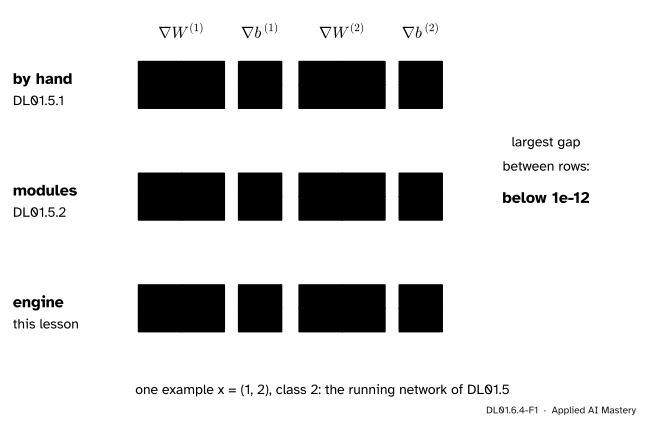
The twelve gradients of the running network of DL01.5, three ways: written out with the chain rule, computed by the module library, and computed by the engine. They agree to rounding.
So the engine is checked against the hand first, one example and then a batch. Only then is it trusted with training, and even there it runs beside the hand-built loop, step for step.
Build it up
Step 1. Copy the weights in. The engine’s Linear stores its weight as (out, in), as DL01.5 does, so the weights of the running network go in without a transpose.
Step 2. One example. Run \({\vect{x} = (1, 2)}\) with class 2 through the engine, call backward, and compare the twelve .grad arrays with the chain-rule lines of DL01.5.1. The input can be a tensor too; its grad is the gradient of the loss with respect to the input.
Step 3. A batch. Run the first eight points of the moons through the engine and through the modules of DL01.5.2. The batch tests everything a single example cannot: broadcasting of the biases, the column sums, and the factor \({1/n}\) of the mean.
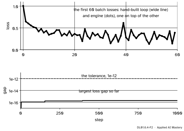
Step 4. A race. Start both from the same weights, feed both the same batches in the same order, and compare their losses at every one of the 1,000 steps of DL01.5.4.
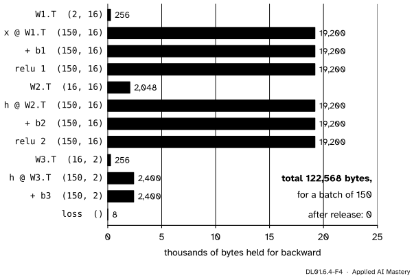
Step 5. Count the memory. A forward pass leaves every intermediate array in the graph, because the closures need them. After backward they are no longer needed.
DL01.6.4-F4
What one forward pass on 150 examples leaves behind. The six activation arrays of shape \({(150, 16)}\) hold almost all of it, and they grow with the batch.
The formal statement
NoteWhat the engine must reproduce, and what it costs
For the running network of DL01.5.1, with \({\vect{\delta}^{(2)}} = {\vect{p}} - {\vect{y}}\) and \({\vect{\delta}^{(1)}} = {(\mat{W}^{(2)\top}\vect{\delta}^{(2)}) \odot [\vect{z}^{(1)} > 0]}\),
\[
\begin{aligned}
\nabla_{\mat{W}^{(2)}} L &= \vect{\delta}^{(2)}\vect{a}^{(1)\top}, \\
\nabla_{\vect{b}^{(2)}} L &= \vect{\delta}^{(2)}, \\
\nabla_{\mat{W}^{(1)}} L &= \vect{\delta}^{(1)}\vect{x}\T, \\
\nabla_{\vect{b}^{(1)}} L &= \vect{\delta}^{(1)} .
\end{aligned}
\]
For a batch of \(n\) examples, a forward pass of this engine keeps three arrays of shape \({(n, n_l)}\) for each hidden layer of width \(n_l\) and two for the output layer, plus the transposed weights, so the memory of training grows linearly with the batch size.
Why the engine must give the same numbers. Each closure of the engine computes one of these products. The fused cross-entropy sends \({(\vect{p} - \vect{y})/n}\) to the logits; the addition of \(\vect{b}^{(2)}\) passes it on and sums it over the batch for the bias; the matrix product sends \({G\mat{W}^{(2)}}\) to the activations and \({\vect{a}^{(1)\top}G}\) towards the weight, which its transpose turns into \({G\T\vect{a}^{(1)}}\) (DL01.6.2); the ReLU applies the mask. With \({n = 1}\) these are the formulas above, written as products of the same numbers, so the results differ by rounding at most.
Why the memory is what it is. A layer of the engine makes three results, \({\mat{W}\T}\), the product and the sum with the bias, and a ReLU makes a fourth; the closures of the next operations read their data. Goodfellow et al. (section 6.5.7) make the same count for a one-hidden-layer network: the memory cost is the stored input to the nonlinearity, of order \({m\,n_h}\) for \(m\) examples and \(n_h\) hidden units. Baydin et al. (section 3.2) note that this storage is the price of reverse mode.
Worked example
The engine’s sweep on the running network, by hand. The forward pass gives \({\vect{z}^{(1)} = (0.5, 1)}\), \({\vect{a}^{(1)} = (0.5, 1)}\), \({\vect{z}^{(2)} = (1, 0)}\), \({\vect{p} \approx (0.731, 0.269)}\) and a loss of about 1.313. Backward:
The fused cross-entropy sends \({\vect{p}} - {\vect{y}} \approx {(0.731, -0.731)}\) to the logits.
The addition of \(\vect{b}^{(2)}\) passes it on, and gives \(\vect{b}^{(2)}\) the same row, since a batch of one has one row to sum.
The product sends \({G\mat{W}^{(2)}}\) to \(\vect{a}^{(1)}\): \({0.731 \cdot (1, 1)} - {0.731 \cdot (-1, 0.5)}
\approx {(1.462, 0.366)}\); and \({G\T\vect{a}^{(1)}}\) to \(\mat{W}^{(2)}\), rows \({0.731 \cdot (0.5, 1)}\) and \({-0.731 \cdot (0.5, 1)}\), about \({(0.366, 0.731)}\) and \({(-0.366, -0.731)}\).
Both pre-activations are positive, so the ReLU passes \({(1.462, 0.366)}\) unchanged; that is the gradient of \(\vect{b}^{(1)}\), and \({G\T\vect{x}}\) gives \(\mat{W}^{(1)}\) the rows \({1.462 \cdot (1, 2)}\) and \({0.366 \cdot (1, 2)}\).
The input gets \({G\mat{W}^{(1)}} \approx {(1.279, -0.366)}\).
Every number is a number of DL01.5.1. Then the race. Both loops start from the weights drawn in DL01.5.4, see its shuffled batches of 32 over 150 training points, and take 200 epochs of five steps at \({\eta = 0.2}\).
DL01.6.4-F2
The race, step for step. Top: the first 60 batch losses of both loops lie on top of each other. Bottom: the largest gap between their losses over all 1,000 steps stays at the size of rounding.
The first batch loss is about 1.005 for both. The largest gap over the whole run stays far below \({10^{-12}}\), at the size of rounding; its exact digits depend on the machine’s arithmetic library, so the code asserts the tolerance, not the digits.
Code
The engine and library of DL01.6.3, and the modules of DL01.5.2, are folded here.
The modules of DL01.5.2 (renamed with an H, for hand)
class HLinear:def__init__(self, W, b):self.W, self.b = np.array(W, float), np.array(b, float)def forward(self, A):self.A = Areturn A @self.W.T +self.bdef backward(self, G):self.dW, self.db = G.T @self.A, G.sum(axis=0)return G @self.Wclass HReLU:def forward(self, Z):self.mask = Z >0return Z *self.maskdef backward(self, G):return G *self.maskclass HSoftmaxCE:def forward(self, Z, labels): Z = Z - Z.max(axis=1, keepdims=True)self.P = np.exp(Z) / np.exp(Z).sum(axis=1, keepdims=True)self.Y = np.eye(Z.shape[1])[labels]return-np.mean(np.log(self.P[np.arange(len(labels)), labels]))def backward(self):return (self.P -self.Y) /len(self.P)class HSequential:def__init__(self, *layers):self.layers = layersdef forward(self, X):for layer inself.layers: X = layer.forward(X)return Xdef backward(self, G):for layer inreversed(self.layers): G = layer.backward(G)return G
The running network of DL01.5.1, by the engine and by the chain-rule lines of that lesson:
W1, b1 = np.array([[1.0, -0.5], [-0.5, 1.0]]), np.array([0.5, -0.5])W2, b2 = np.array([[1.0, 1.0], [-1.0, 0.5]]), np.array([-0.5, 0.0])x, k = np.array([[1.0, 2.0]]), np.array([1]) # class 2 is index 1 in codedef engine_net(values): net = Sequential(Linear(2, 2, np.random.default_rng(0)), ReLU(), Linear(2, 2, np.random.default_rng(0)))for p, value inzip(net.parameters(), values): p.data[...] = value # (out, in) on both sides: no transposereturn netnet = engine_net([W1, b1, W2, b2])xt = Tensor(x)loss = cross_entropy(net(xt), k)loss.backward()engine = [p.grad for p in net.parameters()]# by hand, as in DL01.5.1z1 = W1 @ x[0] + b1; a1 = np.maximum(z1, 0)z2 = W2 @ a1 + b2; p = np.exp(z2 - z2.max()) / np.exp(z2 - z2.max()).sum()d2 = p - np.eye(2)[k[0]]d1 = (W2.T @ d2) * (z1 >0)hand = [np.outer(d1, x[0]), d1, np.outer(d2, a1), d2]print("loss", round(float(loss.data), 3), " grad W1", np.round(engine[0], 3).tolist(), " grad b2", np.round(engine[3], 3).tolist())print("largest gap to the hand:", max(np.abs(e - h).max() for e, h inzip(engine, hand)))print("gradient with respect to the input:", np.round(xt.grad, 3).tolist())
loss 1.313  grad W1 [[1.462, 2.924], [0.366, 0.731]]  grad b2 [0.731, -0.731]
largest gap to the hand: 0.0
gradient with respect to the input: [[1.279, -0.366]]
Then the batch of eight of DL01.5.2, and SciPy’s check_grad on the engine as the library check.
from scipy.optimize import check_gradfrom sklearn.datasets import make_moonsX8, y8 = make_moons(n_samples=200, noise=0.2, random_state=0)X8, y8 = X8[:8], y8[:8]modules = HSequential(HLinear(W1, b1), HReLU(), HLinear(W2, b2))ce = HSoftmaxCE()batch_loss = ce.forward(modules.forward(X8), y8)modules.backward(ce.backward())by_hand = [modules.layers[0].dW, modules.layers[0].db, modules.layers[2].dW, modules.layers[2].db]net8 = engine_net([W1, b1, W2, b2])cross_entropy(net8(Tensor(X8)), y8).backward()by_engine = [p.grad for p in net8.parameters()]print("batch of eight: loss", round(batch_loss, 3), " largest gap", max(np.abs(e - h).max() for e, h inzip(by_engine, by_hand)))def flat_loss(theta): values = [theta[:4].reshape(2, 2), theta[4:6], theta[6:10].reshape(2, 2), theta[10:]]returnfloat(cross_entropy(engine_net(values)(Tensor(X8)), y8).data)def flat_grad(theta): values = [theta[:4].reshape(2, 2), theta[4:6], theta[6:10].reshape(2, 2), theta[10:]] net = engine_net(values) cross_entropy(net(Tensor(X8)), y8).backward()return np.concatenate([p.grad.ravel() for p in net.parameters()])theta = np.concatenate([v.ravel() for v in (W1, b1, W2, b2)])print("check_grad:", f"{check_grad(flat_loss, flat_grad, theta):.1e}")
batch of eight: loss 2.259  largest gap 0.0
check_grad: 3.0e-08
The second row of the first weight’s gradient is zero in both: on these eight points the second hidden unit is dead, as DL01.5.2 found. Now the race: the loop of DL01.5.4, run by the modules and by the engine from the same weights and the same batches.
from sklearn.model_selection import train_test_splitX, y = make_moons(n_samples=200, noise=0.2, random_state=0)X_tr, X_va, y_tr, y_va = train_test_split(X, y, test_size=0.25, stratify=y, random_state=0)rng = np.random.default_rng(0) # the generator of DL01.5.4sizes = [2, 16, 16, 2]start = [(rng.normal(0, np.sqrt(2/ n_in), (n_out, n_in)), np.zeros(n_out))for n_in, n_out inzip(sizes[:-1], sizes[1:])]hand = HSequential(HLinear(*start[0]), HReLU(), HLinear(*start[1]), HReLU(), HLinear(*start[2]))spare = np.random.default_rng(1) # so that rng's next draws are the shuffles of DL01.5.4model = Sequential(Linear(2, 16, spare), ReLU(), Linear(16, 16, spare), ReLU(), Linear(16, 2, spare))for p, value inzip(model.parameters(), [v for pair in start for v in pair]): p.data[...] = valueopt = SGD(model.parameters(), lr=0.2)hand_losses, engine_losses = [], []for epoch inrange(200): order = rng.permutation(len(y_tr))for s inrange(0, len(y_tr), 32): idx = order[s:s +32] ce = HSoftmaxCE() # by hand hand_losses.append(ce.forward(hand.forward(X_tr[idx]), y_tr[idx])) hand.backward(ce.backward())for layer in hand.layers[::2]: layer.W -=0.2* layer.dW layer.b -=0.2* layer.db loss = cross_entropy(model(Tensor(X_tr[idx])), y_tr[idx]) # by the engine engine_losses.append(float(loss.data)) opt.zero_grad() loss.backward() opt.step()hand_losses, engine_losses = np.array(hand_losses), np.array(engine_losses)weight_gap =max(np.abs(h.W - m.weight.data).max() for h, m inzip(hand.layers[::2], model.layers[::2]))with no_grad(): val_acc = np.mean(model(Tensor(X_va)).data.argmax(axis=1) == y_va)print(f"{len(engine_losses)} steps; first loss {engine_losses[0]:.3f}, last {engine_losses[-1]:.3f}")print(f"largest loss gap {np.abs(hand_losses - engine_losses).max():.0e}, largest weight gap {weight_gap:.0e}")print(f"engine-trained validation accuracy {val_acc:.2f}")
1000 steps; first loss 1.005, last 0.008
largest loss gap 2e-16, largest weight gap 2e-15
engine-trained validation accuracy 0.96
Last, the memory. One forward pass on all 150 training points; count the bytes at the result nodes; then free the graph by cutting every node loose from its parents and its closure.
import weakrefdef release(t):"""Drop the graph behind t: every node forgets its parents and its closure."""for node in t.topo_order(): node.parents, node.backward_fn = (), Noneloss = cross_entropy(model(Tensor(X_tr)), y_tr)results = [node for node in loss.topo_order() if node.parents]held =sum(node.data.nbytes for node in results)probe = weakref.ref(max(results, key=lambda node: node.data.size)) # one (150, 16) activationdel resultsloss.backward()release(loss)print(f"{held:,} bytes in the graph before backward; activation still alive after release: {probe() isnotNone}")print("parameter gradients kept:", [p.grad.shape for p in model.parameters()][:2], "...")
122,568 bytes in the graph before backward; activation still alive after release: False
parameter gradients kept: [(16, 2), (16,)] ...
The parameters and their gradients survive; everything the forward pass made is gone at once. The cutting matters in this engine: every result and its closure refer to each other, a reference cycle, so Python would free them only when its cycle collector next runs. PyTorch does the same job inside backward, which frees the graph unless asked to keep it (retain_graph=True).
Explore
The module’s interactive, Broadcast and backward, is in DL01.6.2. Here is what the engine’s training run produced.
DL01.6.4-F3
The 2-16-16-2 network after the engine’s 200 epochs. The boundary bends between the moons exactly as the hand-built network’s did, because it is the same network to the last digits.
Pitfalls
DL01.6.4-F5
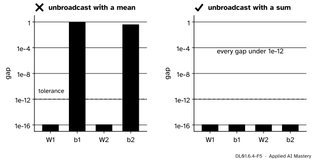
Wrong beside right. With a mean where unbroadcast needs a sum, only the bias gradients are wrong, and a comparison parameter by parameter says so at once.
“The loss goes down, so the gradients are right.”
A wrong gradient still points roughly downhill surprisingly often. The bug in the figure, a mean in place of a sum, divides each bias gradient by the batch size: training still works, only more slowly for the biases. Compare against a reference, parameter by parameter, before trusting a loss curve.
“Agreement to 1e-6 is agreement.”
Two exact methods that compute the same products should agree to within a few units of the last digit, about \({10^{-15}}\) here. A gap of \({10^{-6}}\) between them is a bug, however small it looks: an error of that size is what a finite difference makes, not an exact method.
“Memory is freed as soon as the loss goes out of scope.”
Only if nothing refers to the graph. In this engine results and closures refer to each other, so the graph waits for Python’s cycle collector, and keeping any intermediate tensor in a list (a history of losses as tensors rather than floats, say) keeps its whole graph alive. Store float(loss.data), as the race does, and release the graph after backward.
Check yourself
Recall
1. Why is agreement with the hand-derived gradients a sharper test than central differences?
Show answer
Both are exact methods computing the same products, so they should agree to rounding, about \({10^{-15}}\); a finite difference carries truncation and rounding errors many orders of magnitude larger.
2. What does a batch test that a single example cannot?
Show answer
The broadcasting of the biases with its column sums, and the factor \({1/n}\) of the mean.
3. What must be the same for the engine and the hand-built loop to train step for step?
Show answer
The starting weights, the batches in the same order, the learning rate and the loss; then every step computes the same products.
4. Which arrays hold most of the memory of a forward pass, and how does it grow with the batch?
Show answer
The activations of shape \({(n, n_l)}\) at the hidden layers; it grows linearly with the batch size \(n\).
5. What does release do, and why is it needed in this engine?
Show answer
It clears every node’s parents and closure, so the intermediate arrays are freed at once; without it, the cycles between results and closures wait for the cycle collector.
Exercises
1.★ How many bytes does the engine’s graph hold for one forward pass of the 2-16-16-2 network on a batch of 32, in float64?
Show solution
The transposes hold \({32 + 256 + 32 = 320}\) numbers whatever the batch. The hidden layers make six arrays of shape \({(32, 16)}\), 3,072 numbers; the output layer two of shape \({(32, 2)}\), 128; the loss 1. Total \({320 + 3{,}072 + 128 + 1 = 3{,}521}\) numbers, \({8 \times 3{,}521 = 28{,}168}\) bytes.
2.★★ The bug of the pitfall figure replaces the sum in unbroadcast by a mean. Show that on a batch of \(n\) examples it divides each bias gradient by \(n\) and leaves the weight gradients alone.
Show solution
The bias of shape (out,) is added to a result of shape \({(n, \text{out})}\), so its closure calls unbroadcast on an \({(n, \text{out})}\) gradient, which removes the front axis: a sum gives the column sums, a mean the column sums divided by \(n\). The other argument of that addition, the product, already has shape \({(n, \text{out})}\), so nothing is reduced for it, and the gradient that reaches the weights is unchanged.
3.★★★ A history of losses is kept as tensors, history.append(loss), over 1,000 steps of the race, without release. Estimate the memory this pins in the worst case, and explain why float(loss.data) avoids it.
Show solution
Each loss tensor refers to its parents, and through them to the whole graph of its step: for a batch of 32, about 28 kB (exercise 1) plus the grads that backward allocated for the results, of the same size, so about 56 kB. A thousand of them pin about 56 MB, where one step needs 56 kB. A float is a plain number with no parents, so it keeps nothing else alive, and each step’s graph is freed once the cycle collector runs (or at once with release).
Summary card
An engine is trusted when it matches the hand to rounding, then trains.
DL01.6.4-F1
Three ways, one gradient.
Copy the weights in; compare every gradient, one example and a batch, to about \({10^{-12}}\).
Same weights and batches: the race agrees at every step.
The graph holds the activations, linear in the batch; release it after backward.
From DL01.7 on, PyTorch does this job, and is checked against these numbers.
Sources and next steps
Sources. Each was opened and checked against this lesson on 15 November 2026.
I. Goodfellow, Y. Bengio and A. Courville, Deep Learning, section 6.5.7: for a one-hidden-layer network, backward costs the same order as forward, and the main memory cost is the stored input to the hidden nonlinearity, of order \({m\,n_h}\).
PyTorch 2.15, torch.Tensor.backward: with retain_graph false the graph used to compute the gradients is freed.
A. Karpathy, micrograd: the scalar engine trains a network with two hidden layers of 16 units on the moons; this lesson does the same job with arrays and checks it against hand-derived gradients.
Next.DL01.7.1 Tensors starts the course’s move to PyTorch, which takes over the engine’s job and is checked against the numbers of this module.