One hidden layer of ReLUs draws a curve out of hinges, one bend per unit, so it can follow any continuous curve as closely as you like. Build the network for sin(2 pi x) weight by weight, measure its error, and learn what the universal approximation theorem does not promise.
DL01.2.3L2 Intermediate25 minIn review (what this means)
The maths and code on this page are checked by automated tests on every change, but an independent reader has not signed it off yet. Spot a mistake or a confusing step? Tell us.
Explain why a one-hidden-layer ReLU network computes a continuous piecewise-linear function with one bend per unit.
Construct, weight by weight, the network that interpolates a curve at equally spaced knots.
State the universal approximation theorem and the three things it does not promise.
Measure how the error of the construction falls with the number of units and compare it with a trained network of the same width.
The question
The XOR network needed two hidden units. How far can one hidden layer go if we give it more? Take the wave \({\sin 2\pi x}\) on \({[0, 1]}\): can a network with one hidden layer of ReLUs follow it to within 0.01 everywhere, how many units does that take, and will training find those weights?
From the last lesson
1. How many parameters does a 64-32-10 network have?
Show answer
\({32 \cdot 65 + 10 \cdot 33 = 2410}\).
2. Write one layer of the forward pass for a batch with examples as rows.
Show answer
\({\mat{Z}^{(l)} = \mat{A}^{(l-1)}\mat{W}^{(l)\top} + \vect{1}\,\vect{b}^{(l)\top}}\), then \({\mat{A}^{(l)} = \phi(\mat{Z}^{(l)})}\).
Intuition
Look at one ReLU unit reading a single input \(x\): \({\mathrm{relu}(x - t)}\) is flat until \({x = t}\) and then rises in a straight line. Its graph is a hinge: two straight pieces joined at one bend, the hinge point\(t\). Multiply it by an output weight and it rises or falls at any slope.
Add several hinges with different hinge points and the result is a broken line that bends once at each of them. A network with one hidden layer adds its units exactly like this.
DL01.2.3-F1
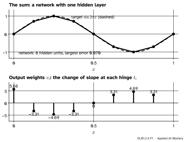
Eight hinges, added up, trace the wave. Each hidden unit bends the line at its hinge point, and its output weight is how much the slope changes there.
More units mean more bends, so shorter straight pieces, and short straight pieces can follow any continuous curve as closely as we like. That is the universal approximation property, seen in one dimension.
Build it up
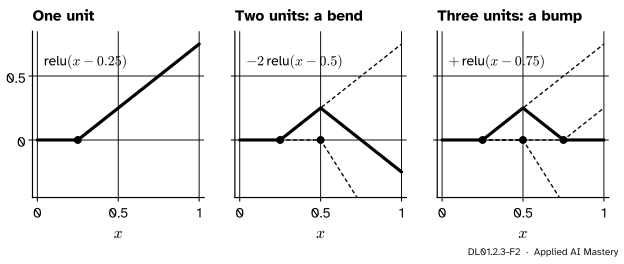
Step 1. One unit.\({\mathrm{relu}(x - 0.25)}\) is 0 up to 0.25 and then has slope 1. In network terms it is a hidden unit with input weight 1 and bias \(-0.25\).
Step 2. Two units make a bend. Add \({-2\,\mathrm{relu}(x - 0.5)}\). Before 0.5 it is 0, so nothing changes there. After 0.5 it adds slope \(-2\), so the total slope turns from 1 to \({1 - 2 = -1}\): the line goes up, then down.
Step 3. Three units make a bump. Add \({\mathrm{relu}(x - 0.75)}\). After 0.75 the slope becomes \({-1 + 1 = 0}\), and the line is flat again, back at 0.
DL01.2.3-F2
Step frames. Each new unit changes the slope at its own hinge point and leaves everything to its left alone. Three units make a bump.
Step 4. The rule. A unit \({v\,\mathrm{relu}(x - t)}\) changes the slope by \(v\) at \(t\) and does nothing to the left of \(t\). So to draw a broken line, put one unit at each bend and set its weight to the change of slope there.
The formal statement
The construction. Choose \(N\) and the equally spaced knots\({t_i = i/N}\) for \({i = 0, 1, \dots, N}\), with \({y_i = f(t_i)}\). On the piece from \(t_i\) to \(t_{i+1}\) the broken line through the knots has slope
\[
s_i = \frac{y_{i+1} - y_i}{t_{i+1} - t_i},
\]
for \({i = 0, \dots, N - 1}\).
Define the network with \(N\) hidden units, input weights 1, biases \(-t_i\), output weights \(v_i\) and output bias \(y_0\):
Claim. For \(x\) in \({[0, 1]}\), \(g\) is the broken line through all \({N + 1}\) knots.
Proof. Take \(x\) in the piece \({[t_k, t_{k+1}]}\). Units with \({i \le k}\) have \({x \ge t_i}\), so they are on and give \({v_i(x - t_i)}\). Units with \({i > k}\) have \({x \le t_i}\) and give 0. So on this piece
\[
g(x) = y_0 + \sum_{i=0}^{k} v_i\,(x - t_i),
\]
a straight line with slope \({v_0 + v_1 + \dots + v_k}\). The sum telescopes: \(s_0 + {(s_1 - s_0)} + \dots + {(s_k - s_{k-1})} = s_k\). At \({x = t_0 = 0}\) every unit is 0, so \({g(t_0) = y_0}\). Moving along piece \(k\) from \(t_k\) to \(t_{k+1}\) with slope \(s_k\) adds \({s_k(t_{k+1} - t_k) = y_{k+1} - y_k}\), so if \({g(t_k) = y_k}\) then \({g(t_{k+1}) = y_{k+1}}\). By induction \(g\) passes through every knot and is straight between them. \(\square\)
How close. For a curve with a bounded second derivative, the broken line through knots a distance \(h\) apart is never further from the curve than
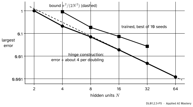
Doubling the units divides the bound by four. For an error below 0.01 it asks for \({\pi^2/(2N^2) < 0.01}\), that is \({N > \pi/\sqrt{0.02} \approx 22.2}\), so 23 units.
Go deeper: proof of the interpolation error bound
Take one piece \({[a, b]}\) with \({b - a = h}\), and write \({e(u) = f(u) - g(u)}\). The broken line meets the curve at the ends, so \({e(a) = e(b) = 0}\). Fix \(x\) strictly between \(a\) and \(b\) and define
Then \({\varphi(a) = \varphi(b) = 0}\), and \({q(x) = 1}\) gives \({\varphi(x) = e(x) - e(x) = 0}\): three zeros. By Rolle’s theorem \(\varphi'\) has a zero between each pair, two zeros in all, and \(\varphi''\) has a zero \(\xi\) between those. On the piece \(g\) is straight, so \({g'' = 0}\) and \({e'' = f''}\), while \({q''(u) = 2/((x - a)(x - b))}\). So
which gives \({e(x) = \tfrac12 f''(\xi)(x - a)(x - b)}\). The product \({(x - a)(b - x)}\) is largest at the middle of the piece, where it is \({h^2/4}\). Hence \({\abs{e(x)} \le \tfrac12 \max\abs{f''} \cdot h^2/4}\), the bound above.
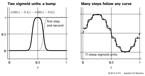
Sigmoids work too. A sigmoid unit \({\sigma(k(x - a))}\) with a large \(k\) is almost a step at \(a\). Two of them make a bump: \({\sigma(k(x - a)) - \sigma(k(x - b))}\) is near 1 between \(a\) and \(b\) and near 0 elsewhere. Bumps of the right heights side by side make a staircase that follows any continuous curve.
DL01.2.3-F4
With sigmoids, two steep units make a bump, and many steps follow a curve. This shows why the theorem is plausible; Cybenko’s proof is different and does not construct the units.
NoteThe universal approximation theorem
Let \(f\) be continuous on a closed and bounded set \(K\) in \(\R^d\) and let \({\varepsilon > 0}\). Then there is a network with one hidden layer, finitely many units and a linear output,
with \({\abs{G(\vect{x}) - f(\vect{x})} < \varepsilon}\) for every \(\vect{x}\) in \(K\). Cybenko (1989) proved it for continuous sigmoidal \(\phi\) on the unit cube, Hornik (1991) for every continuous, bounded, non-constant \(\phi\), and Leshno, Lin, Pinkus and Schocken (1993) for every locally bounded, piecewise continuous \(\phi\) that is not a polynomial, which includes the ReLU.
Three things the theorem does not say:
How many units. It promises a finite number, not a small one. In one dimension the hinge construction needs about \({\pi/\sqrt{2\varepsilon}}\) units for the sine; for a function of many inputs the number can grow exponentially with \(d\) (Goodfellow et al., section 6.4.1).
That training finds them. The weights exist; gradient descent may stop elsewhere. The code below shows it.
That they generalise. The theorem is about matching a known \(f\) everywhere. Learning works from finitely many noisy examples, and a network that fits them need not fit new ones (ML01.8).
Worked example
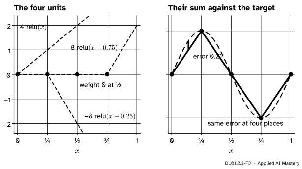
Build the network for \({N = 4}\). The knots are \({0, \tfrac14, \tfrac12, \tfrac34, 1}\) and the values of \({\sin 2\pi x}\) there are \({0, 1, 0, -1, 0}\).
Slopes. Each piece has width \(\tfrac14\), so each slope is 4 times the change in value:
The unit at \(\tfrac12\) has weight 0: the line does not bend there, because the pieces on both sides have the same slope.
Check a knot. At \({x = \tfrac12}\): \({4 \cdot \tfrac12 - 8 \cdot \tfrac14 + 0 = 2 - 2 = 0}\), which is \({\sin \pi = 0}\).
DL01.2.3-F3
The four-unit network, built weight by weight. Its largest error, 0.21, occurs at four places, one in each quarter, because the wave is symmetric.
The largest error. On the first piece \({g(x) = 4x}\) and the error is \({e(x) = \sin 2\pi x - 4x}\). It is largest where \({e'(x) = 2\pi\cos 2\pi x - 4 = 0}\), that is \({\cos 2\pi x = 2/\pi}\), at \({x \approx 0.140}\). There \({\sin 2\pi x = \sqrt{1 - 4/\pi^2} \approx 0.771}\) and \({4x \approx 0.561}\), so the error is about 0.211. The bound promised at most \({\pi^2/32 \approx 0.308}\).
Code
The construction from scratch, and its largest error measured on a fine grid.
import numpy as npdef f(x):return np.sin(2* np.pi * x)def hinge_network(N):"""Hinge points t_i, output weights v_i and output bias of the N-unit interpolating network.""" t = np.arange(N +1) / N s = np.diff(f(t)) / np.diff(t) # slope of each piece v = np.diff(np.concatenate([[0.0], s])) # change of slope at each hingereturn t[:-1], v, f(t[0])def g(x, t, v, c):return c + np.maximum(x[:, None] - t, 0.0) @ v # one column per hidden unitxs = np.linspace(0, 1, 100001)t4, v4, c4 = hinge_network(4)print("N = 4 output weights:", (np.round(v4, 6) +0.0).tolist()) # + 0.0 turns -0.0 into 0.0errors = {}for N in (4, 8, 16, 32): errors[N] =float(np.max(np.abs(g(xs, *hinge_network(N)) - f(xs))))print(f"N = {N:2d}: largest error {errors[N]:.4f}, bound {np.pi**2/ (2* N**2):.4f}")smallest =next(N for N inrange(1, 100) if np.max(np.abs(g(xs, *hinge_network(N)) - f(xs))) <0.01)print("fewest units for an error below 0.01:", smallest)
N = 4 output weights: [4.0, -8.0, 0.0, 8.0]
N =  4: largest error 0.2105, bound 0.3084
N =  8: largest error 0.0704, bound 0.0771
N = 16: largest error 0.0188, bound 0.0193
N = 32: largest error 0.0048, bound 0.0048
fewest units for an error below 0.01: 23
From 8 units on, each doubling of \(N\) divides the error by close to four, as the bound says (from 4 to 8 it falls by a factor of 3, because 4 pieces are too coarse for the bound to be sharp). 23 units are the fewest that get below 0.01.
DL01.2.3-F5
The construction falls on a straight line of slope \(-2\) on log-log axes. Networks of the same width trained by scikit-learn stay well above it, even the best of ten starting points.
Now train networks of the same widths with scikit-learn’s MLPRegressor, whose output layer is the identity, on 200 evenly spaced points of the curve. We switch its L2 penalty off (alpha=0) and give it ten random starts.
import warningsfrom sklearn.neural_network import MLPRegressorx_train = np.linspace(0, 1, 200)[:, None]grid = np.linspace(0, 1, 2001)trained = {}with warnings.catch_warnings(): warnings.simplefilter("ignore")for N in (4, 8, 16, 32): runs = []for seed inrange(10): net = MLPRegressor(hidden_layer_sizes=(N,), activation="relu", solver="lbfgs", alpha=0.0, max_iter=10000, tol=1e-12, max_fun=100000, random_state=seed) net.fit(x_train, f(x_train.ravel())) runs.append(float(np.max(np.abs(net.predict(grid[:, None]) - f(grid))))) trained[N] = runsprint(f"N = {N:2d}: best of 10 {min(runs):.3f}, worst {max(runs):.3f}, construction {errors[N]:.4f}")
N =  4: best of 10 0.908, worst 1.132, construction 0.2105
N =  8: best of 10 0.185, worst 1.132, construction 0.0704
N = 16: best of 10 0.079, worst 1.133, construction 0.0188
N = 32: best of 10 0.035, worst 0.196, construction 0.0048
At every width the best trained network is several times worse than the construction, and some starts end with an error near 1, as bad as predicting 0 everywhere. The exact figures can move a little between machines; the gap does not.
Explore
The left half of the module’s interactive, hinges and folds, in lesson DL01.2.4, is this construction: drag up to a dozen knots and watch the network follow \({\sin 2\pi x}\), with its largest error printed.
Pitfalls
DL01.2.3-F6
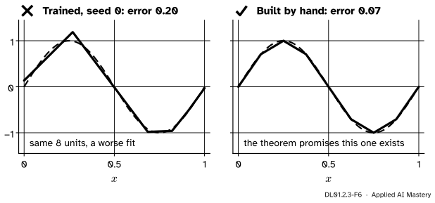
Wrong beside right. Both networks have eight hidden units. Training from a random start found a worse fit than the one we can write down.
“The theorem says a neural network will learn any function.”
It says a network that approximates the function exists. Finding its weights is an optimisation problem with no guarantee, and the loss of a network has many poor stopping points (DL01.4.4). The eight-unit networks above all could reach an error of 0.07; none of ten training runs did.
“One hidden layer is enough, so depth is pointless.”
Enough in principle, not in size. The construction needs a unit per bend, and some functions have a great many bends. The next lesson shows a function that four layers of two units compute exactly and that one hidden layer needs 16 units to match.
“A good approximation of the training points is a good model.”
The theorem is about matching a function everywhere, with the whole function known. A network that passes through every training point can still be far off between them. Judge a trained network on held-out data (ML01.2), never on the theorem.
Check yourself
Recall
1. What does the graph of a single unit \({v\,\mathrm{relu}(x - t)}\) look like?
Show answer
A hinge: flat at 0 up to \({x = t}\), then a straight line of slope \(v\).
2. In the hinge construction, what is the output weight of the unit at knot \(t_i\)?
Show answer
The change of slope there, \({v_i = s_i - s_{i-1}}\), with \({v_0 = s_0}\).
3. How does the error of the construction for \({\sin 2\pi x}\) change when \(N\) doubles?
Show answer
Once \(N\) is not tiny it falls by close to a factor of 4, following the bound \({\pi^2/(2N^2)}\).
4. State the universal approximation theorem in one sentence.
Show answer
Any continuous function on a closed and bounded set can be matched to within any \({\varepsilon > 0}\) by a network with one hidden layer of enough units, for any non-polynomial activation of the usual kinds.
5. Name the three things the theorem does not promise.
Show answer
How many units are needed, that training will find the weights, and that the network will generalise from finitely many examples.
Exercises
1.★ Build the hinge network for \({f(x) = x^2}\) on \({[0, 1]}\) with \({N = 2}\). Give its weights and its value at \({x = 0.25}\).
Show solution
Knots 0, 0.5, 1 with values 0, 0.25, 1. Slopes \({s_0 = 0.25/0.5 = 0.5}\) and \({s_1 = 0.75/0.5 = 1.5}\). So \({v_0 = 0.5}\), \({v_1 = 1.5 - 0.5 = 1}\), bias 0, and \(g(x) = {0.5\,\mathrm{relu}(x)} + {\mathrm{relu}(x - 0.5)}\). At 0.25 only the first unit is on: \({g(0.25) = 0.125}\), against \({f(0.25) = 0.0625}\). The bound \({h^2/8} \cdot {\max\abs{f''}} = {0.25/8} \cdot 2 = 0.0625\) is met exactly here.
2.★★ Use the bound to find how many units guarantee an error below 0.001 for \({\sin 2\pi x}\).
Show solution
We need \({\pi^2/(2N^2) < 0.001}\), so \({N^2 > 500\pi^2}\) and \({N > \pi\sqrt{500} \approx 70.2}\). 71 units suffice. Ten times less error costs about \({\sqrt{10} \approx 3.2}\) times as many units.
3.★★★ Show that a network with one hidden layer of \(n\) ReLU units and one input computes a function with at most \({n + 1}\) linear pieces on the whole real line.
Show solution
Each unit \({v\,\mathrm{relu}(wx + b)}\) with \({w \ne 0}\) is linear on each side of the single point \({x = -b/w}\); with \({w = 0}\) it is constant. The output is a sum of such functions plus a constant, so it is linear on any interval that contains none of these points. There are at most \(n\) points, and \(n\) points cut the line into at most \({n + 1}\) intervals. On each interval the output is one straight piece, so there are at most \({n + 1}\) pieces.
Summary card
One hidden layer of ReLUs draws a broken line, one bend per unit.
Error. At most \({\tfrac{h^2}{8}\max\abs{f''}}\), which is \({\pi^2/(2N^2)}\) for \({\sin 2\pi x}\).
Theorem. One hidden layer can match any continuous function on a closed bounded set.
Not promised. The number of units, that training finds them, that they generalise.
Sources and next steps
Sources. Each was opened and checked against this lesson on 15 November 2026.
Simon J. D. Prince, Understanding Deep Learning, MIT Press, free PDF. Section 3.2 shows that a shallow ReLU network with \(D\) hidden units has at most \(D\) joints and \({D + 1}\) linear regions, and approximates a 1D function better as the regions grow more numerous (figure 3.5). The notes to chapter 3 credit the width version of the theorem to Cybenko (1989) for sigmoids and to Hornik (1991) for a larger class of activations.
Ian Goodfellow, Yoshua Bengio and Aaron Courville, Deep Learning, section 6.4.1. States the theorem for continuous functions on a closed and bounded subset of \(\R^n\), notes that Leshno et al. (1993) extended it to rectified linear units, and lists what it does not guarantee: the training algorithm may fail to find the weights or may overfit, and the network may need exponentially many units.
George Cybenko, Approximation by superpositions of a sigmoidal function, Mathematics of Control, Signals, and Systems 2 (1989), 303 to 314. Theorem 2: for any continuous sigmoidal function, finite sums of the form used above are dense in the continuous functions on the unit cube.
Moshe Leshno, Vladimir Lin, Allan Pinkus and Shimon Schocken, Multilayer feedforward networks with a nonpolynomial activation function can approximate any function, Neural Networks 6 (1993), 861 to 867. Theorem 1 gives the condition “not a polynomial” for locally bounded, piecewise continuous activations; the introduction quotes Hornik’s (1991) theorem for continuous, bounded, non-constant activations on compact sets.