Stack layers into a multilayer perceptron: each one a matrix product, a bias and an activation. Count its parameters, run its forward pass by hand and for a whole batch, then reproduce scikit-learn’s MLPClassifier from its fitted weights.
DL01.2.2L2 Intermediate25 minIn review (what this means)
The maths and code on this page are checked by automated tests on every change, but an independent reader has not signed it off yet. Spot a mistake or a confusing step? Tell us.
Write the forward pass of a multilayer perceptron layer by layer, for one example and for a batch with examples as rows.
Count the parameters of a network from its layer sizes, each layer holding its width times one more than the width before it.
Carry out the forward pass of a small network by hand.
Implement a forward function for any list of layer sizes and check it against scikit-learn’s fitted MLPClassifier.
The question
The digit classifier at the end of this course is described by three numbers, 64-32-10. From those three numbers alone you can say exactly how an image flows through it and that it holds 2,410 adjustable numbers. How, and what do the three numbers leave out?
From the last lesson
1. Where does the hidden layer of the hand-built XOR network send \({(0, 1)}\) and \({(1, 0)}\)?
Show answer
Both to \({(1, 0)}\), because both have \({x_1 + x_2 = 1}\).
2. Why must a hidden layer have an activation to help with XOR?
Show answer
Without one, the layers compose into a single affine map, which is no stronger than one neuron.
Intuition
A multilayer perceptron (MLP) is a chain of layers. Each layer is the layer of DL01.1.3: a matrix product, a bias and an activation. Its output becomes the next layer’s input. The XOR network of the last lesson had one hidden layer. Nothing stops us from stacking more.
DL01.2.2-F1
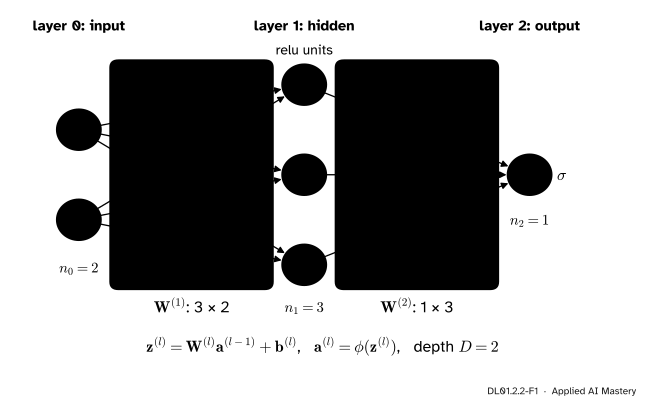
A 2-3-1 multilayer perceptron. Every unit of a layer reads every unit of the layer before, so the weights between two layers form one matrix, with a row for each unit it feeds.
Three words describe the shape of such a network. The width of a layer is its number of units, \(n_l\). The depth\(D\) is the number of weight layers, so the network in the figure has depth 2: the input is layer 0 and holds no weights. The list of widths, here 2-3-1, is the architecture. It fixes the shape of every weight matrix, and so the number of parameters, but not their values: those come from training.
Build it up
Step 1. One layer. Layer \(l\) takes the activations \(\vect{a}^{(l-1)}\) of the layer before, multiplies by its weight matrix, adds its bias and applies the activation: \({\vect{a}^{(l)} = \phi(\mat{W}^{(l)}\vect{a}^{(l-1)} + \vect{b}^{(l)})}\). The input is \({\vect{a}^{(0)} = \vect{x}}\).
Step 2. The shape of a weight matrix. Row \(j\) of \(\mat{W}^{(l)}\) holds the weights of unit \(j\) of layer \(l\), one for each unit of layer \({l - 1}\). So \(\mat{W}^{(l)}\) has \(n_l\) rows and \(n_{l-1}\) columns: shape (out, in), the shape PyTorch’s nn.Linear stores.
Step 3. Chain the layers. Run layer 1 on \(\vect{x}\), layer 2 on its output, and so on to layer \(D\). The last layer’s activation depends on the task: the identity for a number, the sigmoid for a probability of one class (as here), the softmax for several classes (DL01.4).
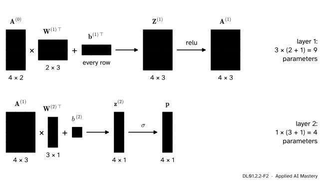
Step 4. A batch at once. With \(n\) examples as the rows of a matrix, one matrix product does a whole layer for every example.
DL01.2.2-F2
The forward pass for a batch of four, drawn to shape. Each layer is one matrix product, one added row and one activation. The inner sizes always match: 2 with 2, then 3 with 3.
The formal statement
NoteDefinition: multilayer perceptron
A multilayer perceptron of depth \(D\) with widths \({n_0 = d, n_1, \dots, n_D}\) has, for each layer \({l = 1, \dots, D}\), a weight matrix \(\mat{W}^{(l)}\) of shape \(n_l\) by \(n_{l-1}\) and a bias \(\vect{b}^{(l)}\) in \(\R^{n_l}\). Its forward pass starts from \({\vect{a}^{(0)} = \cdata{\vect{x}}}\) and computes, for \({l = 1, \dots, D}\),
The output is \(\cmodel{\vect{a}^{(D)}}\), where the last layer may use its own activation.
Counting parameters. Layer \(l\) owns \(\mat{W}^{(l)}\), which has \({n_l \times n_{l-1}}\) entries, and \(\vect{b}^{(l)}\), which has \(n_l\). Together that is \({n_l n_{l-1} + n_l}\), and taking out the common factor,
\[
\begin{aligned}
&\text{parameters of layer } l \\
&\quad= n_l\,(n_{l-1} + 1).
\end{aligned}
\]
The “+ 1” is the bias: one extra weight per unit. Add up the layers:
For 2-3-1 that is \({3 \cdot 3 + 1 \cdot 4 = 13}\). For the digit network 64-32-10 it is \({32 \cdot 65} + {10 \cdot 33} = 2080 + 330 = 2410\), the number in the question.
The batch form. Put the \(n\) examples in the rows of a matrix \(\mat{A}^{(0)}\) of shape \(n\) by \(d\). Row \(i\) of the layer’s result should be the transpose of the single-example result for example \(i\). Transposing \({\mat{W}\vect{a}_i + \vect{b}}\) reverses the product:
Stacking these rows for \({i = 1, \dots, n}\) gives the course’s batch layer, with \(\vect{1}\) the column of \(n\) ones that copies the bias into every row:
The shapes check: \(n\) by \(n_{l-1}\) times \(n_{l-1}\) by \(n_l\) is \(n\) by \(n_l\), one row per example and one column per unit. Then \({\mat{A}^{(l)} = \phi(\mat{Z}^{(l)})}\), entry by entry. In NumPy the term \({\vect{1}\,\vect{b}\T}\) is written + b, and broadcasting adds the bias to every row.
Go deeper: what the architecture leaves out
The widths fix the shapes, but four more choices complete a network: the hidden activation, the output activation, the loss (DL01.4) and how the weights start (DL02.3). Two networks with the same widths and different activations compute different families of functions. The widths also say nothing about how layers are wired beyond “each reads the one before”: skip connections (DL02.7) and convolutions (DL03) change that.
Worked example
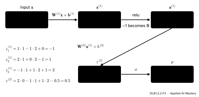
Take the 2-3-1 network of the figure with ReLU hidden units and a sigmoid output, and these weights:
The forward pass of one example, every number written out. The first hidden unit is switched off for this input, so its weight 2 into the output has no effect.
Layer 1. Each row of \(\mat{W}^{(1)}\) meets the input, then the bias is added:
Output.\({p = \sigma(0.5) = 1/(1 + e^{-0.5}) \approx 0.622}\). The network gives this input a 62 percent chance of being in class 1.
The network has \({9 + 4 = 13}\) parameters, and this one input used them all except the weight from the switched-off unit: whatever that weight were, \(p\) would be the same. That is why, in backpropagation (DL01.5), a unit that is off passes no gradient back to its outgoing weight.
Code
A forward pass for any list of layer sizes, from scratch. The weights are stored (out, in), as in the course, and the examples are rows.
import numpy as npdef relu(z):return np.maximum(z, 0.0)def sigmoid(z):return1.0/ (1.0+ np.exp(-z))def init(sizes, seed=0):"""Random weights of shape (out, in) and zero biases for the widths in `sizes`.""" rng = np.random.default_rng(seed)return [(rng.normal(0, 1/ np.sqrt(n_in), (n_out, n_in)), np.zeros(n_out))for n_in, n_out inzip(sizes[:-1], sizes[1:])]def forward(A, layers):"""ReLU hidden layers and a sigmoid output; A has one example per row."""for l, (W, b) inenumerate(layers, start=1):assert A.shape[1] == W.shape[1], f"layer {l}: input width {A.shape[1]}, W expects {W.shape[1]}" Z = A @ W.T + b A = relu(Z) if l <len(layers) else sigmoid(Z)return Adef n_params(sizes):returnsum(n_out * (n_in +1) for n_in, n_out inzip(sizes[:-1], sizes[1:]))layers = [(np.array([[1.0, -1.0], [2.0, 0.0], [-1.0, 1.0]]), np.array([0.0, -1.0, 1.0])), (np.array([[2.0, -1.0, 1.0]]), np.array([-0.5]))]p = forward(np.array([[1.0, 2.0]]), layers)print("worked example: p =", round(float(p[0, 0]), 3))print("parameters:", n_params([2, 3, 1]), n_params([64, 32, 10]), n_params([2, 16, 16, 1]))print("a batch of 5 through 64-32-10:", forward(np.ones((5, 64)), init([64, 32, 10])).shape)
worked example: p = 0.622
parameters: 13 2410 337
a batch of 5 through 64-32-10: (5, 10)
Now scikit-learn. MLPClassifier trains a network of this kind; we fit it to the course’s moons and then recompute its probabilities with our own forward. One detail matters: scikit-learn stores the weights between layer \(l\) and layer \({l + 1}\) in coefs_[l] with shape (in, out), the transpose of ours.
from sklearn.datasets import make_moonsfrom sklearn.neural_network import MLPClassifierX, y = make_moons(n_samples=200, noise=0.2, random_state=0)clf = MLPClassifier(hidden_layer_sizes=(16, 16), solver="lbfgs", max_iter=2000, random_state=0).fit(X, y)print("stored shapes:", [W.shape for W in clf.coefs_], " output:", clf.out_activation_)ours = [(W.T, b) for W, b inzip(clf.coefs_, clf.intercepts_)] # transpose once, on loadingp_ours = forward(X, ours).ravel()p_sklearn = clf.predict_proba(X)[:, 1]print("largest difference:", float(np.max(np.abs(p_ours - p_sklearn))))print("training accuracy:", round(float(np.mean((p_ours >=0.5) == y)), 3))
stored shapes: [(2, 16), (16, 16), (16, 1)]  output: logistic
largest difference: 0.0
training accuracy: 0.965
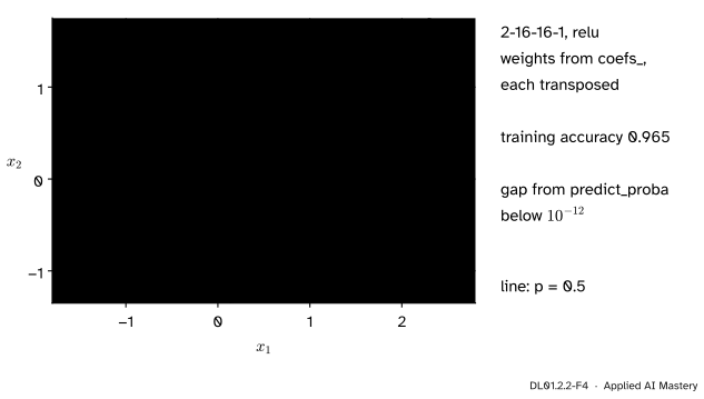
The two agree to at least twelve decimal places, so our forward pass is the network scikit-learn trained. Its training accuracy is about 0.97 (the last digit can differ on another machine). Its boundary, drawn by our function, is below.
DL01.2.2-F4
The decision boundary of scikit-learn’s fitted network, computed by our own forward pass from coefs_ and intercepts_.
Explore
The module’s interactive, hinges and folds, lives in lesson DL01.2.4. Its right half is a deep network of exactly this kind, with two units per layer, and a depth slider.
Pitfalls
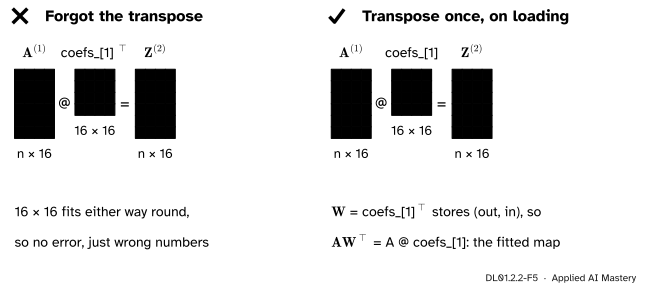
DL01.2.2-F5
Wrong beside right. A square weight matrix multiplies without complaint whichever way round it is, so a missing transpose raises no error. Only the numbers are wrong.
“If the shapes fit, the weights are the right way round.”
Shape checks catch a missing transpose only when a layer is not square. The middle layer of the 2-16-16-1 network is 16 by 16, and using coefs_[1] where \(\mat{W}\) belongs runs silently. The next cell shows how far the probabilities move. Convert a library’s weights once, when loading them, and compare outputs, not just shapes.
wrong = [ours[0], (clf.coefs_[1], clf.intercepts_[1]), ours[2]] # middle layer not transposedp_wrong = forward(X, wrong).ravel()print("largest change in a probability:", round(float(np.max(np.abs(p_wrong - p_ours))), 2))
largest change in a probability: 1.0
“A 2-3-1 network has three layers, so its depth is 3.”
The input is layer 0 and owns no weights. Depth counts weight layers, so 2-3-1 has depth 2 and one hidden layer. Counting the input inflates every depth by one and every comparison of depths in DL01.2.4 with it. Some books, Prince’s among them, count hidden layers instead, which gives 1 here; whichever count a text uses, check it before comparing depths across texts.
“A layer from 3 units to 1 has 3 parameters.”
It has 4: three weights and one bias. Forgetting the “+ 1” in \({n_l(n_{l-1} + 1)}\) undercounts every layer by its width. For 64-32-10 it would give 2,368 instead of 2,410.
Check yourself
Recall
1. What shape does \(\mat{W}^{(l)}\) have, and what does row \(j\) hold?
Show answer
\(n_l\) by \(n_{l-1}\), that is (out, in). Row \(j\) holds the weights of unit \(j\) of layer \(l\), one per unit of the layer before.
2. Write the batch form of one layer and say what the column of ones does.
Show answer
\({\mat{Z}^{(l)} = \mat{A}^{(l-1)}\mat{W}^{(l)\top} + \vect{1}\,\vect{b}^{(l)\top}}\); the column of ones copies the bias into every row, one row per example.
3. How many parameters does a network with widths 64-32-10 have, and how is the number found?
3: there are three weight matrices. It has two hidden layers.
5. In what shape does scikit-learn store the weights in coefs_, and what must you do before using them in the course’s forward pass?
Show answer
Each coefs_[l] has shape (in, out); transpose it to get the course’s (out, in) matrix.
Exercises
1.★ Count the parameters of the network 784-256-128-10, layer by layer.
Show solution
Layer 1: \({256 \cdot 785 = 200{,}960}\). Layer 2: \({128 \cdot 257 = 32{,}896}\). Layer 3: \({10 \cdot 129 = 1{,}290}\). The total is 235,146, and most of it is the first layer, because the input is wide.
2.★★ Run the worked example’s network on \({\vect{x} = (2, 1)}\) by hand. Which hidden unit is off this time?
Show solution
\({z^{(1)}_1 = 2 - 1 + 0 = 1}\), \({z^{(1)}_2 = 4 + 0 - 1 = 3}\) and \({z^{(1)}_3 = -2 + 1 + 1 = 0}\), so \({\vect{a}^{(1)} = (1, 3, 0)}\). The third unit is off (its pre-activation is exactly 0). Then \(z^{(2)} = {2 \cdot 1} - {1 \cdot 3} + {1 \cdot 0} - 0.5 = -1.5\) and \({p = \sigma(-1.5) \approx 0.182}\).
3.★★★ A network has 10 inputs, three hidden layers of the same width \(w\) and one output. Show that it has \({2w^2 + 14w + 1}\) parameters, and find the largest \(w\) that keeps it within 10,000.
Show solution
The layers give \({w(10 + 1)}\), then twice \({w(w + 1)}\), then \({1 \cdot (w + 1)}\). Adding them:
For \({w = 67}\) this is \({8978 + 938 + 1 = 9917}\). For \({w = 68}\) it is \({9248 + 952 + 1 = 10{,}201}\), too many. So \({w = 67}\). The count grows with the square of the width, which is why wide hidden layers are expensive.
Summary card
A multilayer perceptron is a chain of matrix product, bias, activation.
DL01.2.2-F1
Widths 2-3-1, depth 2.
One layer.\({\vect{z}^{(l)} = \mat{W}^{(l)}\vect{a}^{(l-1)} + \vect{b}^{(l)}}\), \({\vect{a}^{(l)} = \phi(\vect{z}^{(l)})}\), with \(\mat{W}^{(l)}\) of shape (out, in).
A batch.\({\mat{Z}^{(l)} = \mat{A}^{(l-1)}\mat{W}^{(l)\top} + \vect{1}\,\vect{b}^{(l)\top}}\), examples as rows.
Parameters.\({\sum_l n_l(n_{l-1} + 1)}\); 64-32-10 has 2,410.
Depth. The number of weight layers; the input is layer 0.
Sources and next steps
Sources. Each was opened and checked against this lesson on 15 November 2026.
Ian Goodfellow, Yoshua Bengio and Aaron Courville, Deep Learning, chapter 6, MIT Press. The introduction to chapter 6 describes a feedforward network as a chain of functions whose length is its depth; section 6.4 on architecture design writes each layer of a chain as an activation of a weight matrix times the layer before plus a bias (equation 6.40).
Simon J. D. Prince, Understanding Deep Learning, MIT Press, free PDF. Section 4.3.1 names width and depth as hyperparameters chosen before training (Prince counts hidden layers, where this course counts weight layers), and section 4.4 writes a deep network in matrix notation, one layer at a time.
scikit-learn developers, Neural network models (supervised), section 1.17, and the MLPClassifier reference, version 1.9.1. coefs_[i] holds the weights between layer \(i\) and layer \({i + 1}\) and intercepts_[i] the biases added to layer \({i + 1}\); the binary output passes through the logistic function; the defaults are a relu activation, the adam solver and an L2 penalty alpha of 0.0001. The shape (in, out) of each matrix is checked in the code above.
Next.DL01.2.3 Universal approximation asks how much one hidden layer can do, and answers: any continuous curve, if it is wide enough.