Before any network is trained, say what the task is, how it will be scored and what score would count as success. Examine the 1,797 digit images, score with accuracy and per-class recall, and set two baselines on the validation set: the majority class and logistic regression.
DL01.10.1L2 Intermediate25 minIn review (what this means)
The maths and code on this page are checked by automated tests on every change, but an independent reader has not signed it off yet. Spot a mistake or a confusing step? Tell us.
State the task, the input, the output and the score of the digit project in one sentence each.
Derive that accuracy is the average of the per-class recalls weighted by the class shares, and use it to explain why accuracy suits balanced classes.
Compute the majority-class baseline by hand from class counts, including how a tie is broken.
Fit a logistic-regression baseline on the scaled pixels and report its validation accuracy and per-class recall.
The question
You have 1,797 tiny pictures of handwritten digits and a network design that can learn from them. Before you train anything: what number will you look at to judge the network, and how high must it be before the network has earned its place?
Intuition
A project does not start with a model. It starts with a sentence: given an 8 by 8 image of a handwritten digit, say which of the ten digits it is. Then a score, and then a bar: the score that a much simpler method already reaches. A network that does not clear the bar has not earned its extra complexity, however good its number looks on its own.
DL01.10.1-F1
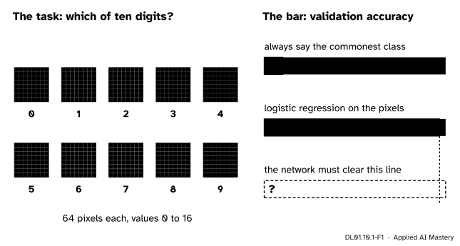
The project in one picture. The input is 64 pixel values, the answer one of ten classes, and two baselines measured on the validation images set the bar before any network is trained.
Two baselines set the bar. The first is the dumbest rule there is: always answer the most common class. It shows what “no learning at all” scores. The second is a good simple model, logistic regression on the raw pixels (ML01.6): one linear layer and a softmax, no hidden layer. It shows what a hidden layer has to add. In this project the second bar is high, and that is the useful surprise of this lesson.
Build it up
Step 1. The images.load_digits ships with scikit-learn, so nothing is downloaded. Each image began as a 32 by 32 black-and-white bitmap; the dataset cuts it into 64 blocks of 4 by 4 and counts the black pixels in each block. So every value is a count from 0 to 16, and an image is 64 such counts. About half of all the values are 0, the white background.
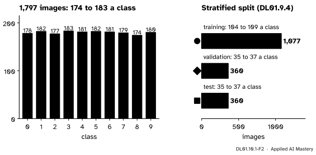
Step 2. The classes. Ten digits, with 174 to 183 images each: the classes are balanced, nearly equal in size. The split of DL01.9.4 keeps those shares in each part: 1,077 training, 360 validation and 360 test images, with 104 to 109, 35 to 37 and 35 to 37 images of each class.
DL01.10.1-F2
The classes are nearly equal in size, and the stratified split keeps every class’s share in the training, validation and test images.
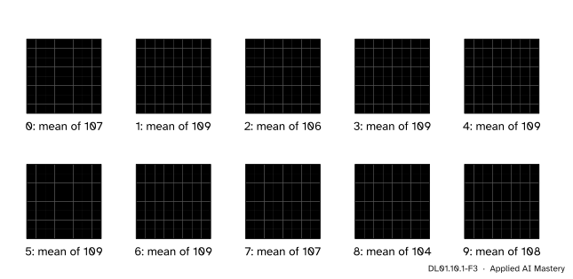
Step 3. What a class looks like. Average the training images of one class, pixel by pixel, and the mean image already looks like its digit. That tells us something before any training: the pixels carry the answer in a fairly direct way, so even a linear model should do well.
DL01.10.1-F3
The mean training image of each class. Each is already recognisable: the information is sitting in the pixels.
Step 4. Scale the pixels. Dividing every value by 16 puts the inputs in \([0, 1]\). The constant 16 is fixed by how the data were made, not estimated from the data, so dividing by it cannot leak anything from the validation or test images into training (the leak of ML01.2.4 comes from statistics computed on all the data).
Step 5. The score. The classes are balanced, so the plain accuracy, the share of images classified correctly, is a fair summary. Beside it we report the recall of each class, the share of that class’s images that are classified correctly, so that one weak class cannot hide.
The formal statement
NoteAccuracy and per-class recall
For \(n\) images with true classes \(y_i\) and predictions \(\hat{y}_i\), let \(n_k\) be the number of images of class \(k\) and \(r_k\) the number of those that are classified correctly. The accuracy is \({A = \tfrac{1}{n} \sum_k r_k}\) and the recall of class \(k\) is \({R_k = r_k / n_k}\). Then
\[
A = \sum_{k=0}^{9} \frac{n_k}{n}\, R_k ,
\]
the average of the recalls, each weighted by its class’s share of the images.
Derivation. Every correctly classified image belongs to exactly one class, so the number right is the sum over classes, \({r_0 + r_1 + \dots + r_9}\). Multiply and divide each term by its own \(n_k\):
ML01.7.1 did this for two classes; nothing changes with ten.
Two consequences. First, a classifier that always answers class \(m\) has \({R_m = 1}\) and \({R_k = 0}\) for every other class, so its accuracy is \({n_m / n}\), the share of the class it names. The best constant answer is the most common class, and it scores the largest share. With balanced classes that share is close to \({1/K}\), here about 10 percent.
Second, when every share \({n_k / n}\) is close to \({1/K}\), accuracy is close to the plain mean of the recalls (the balanced accuracy of ML01.7.1), so no class can drag the accuracy far from what each class sees. On our validation set the shares are 35, 36 or 37 out of 360, all within \({1/360}\) of \({0.1}\). With badly imbalanced classes the weights differ, a big class dominates, and accuracy can look excellent while a small class fails: there, report the recalls first.
Worked example
The majority baseline, by hand. The rule is fitted on the training images, as every model is, and scored on the validation images.
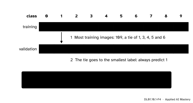
Count the training images of each class: 107, 109, 106, 109, 109, 109, 109, 107, 104 and 108 for the classes 0 to 9.
The largest count is 109, shared by five classes: 1, 3, 4, 5 and 6. scikit-learn’s DummyClassifier takes the first of them, so the rule says “1” for every image.
The validation set holds 37 images of class 1, so the rule is right 37 times in 360: \({37 / 360 = 0.103}\).
DL01.10.1-F4
The majority baseline traced from the training counts to its validation accuracy.
Check it with the formula: the recall of class 1 is 1 and every other recall is 0, so \({A = \tfrac{37}{360} \cdot 1 = 0.103}\).
The logistic-regression baseline. It is fitted on the 1,077 scaled training images and gets 348 of the 360 validation images right: \({348/360 = 0.967}\). Its lowest recalls are 0.943, for class 0 (33 of 35) and class 8 (33 of 35). Weighted by the shares, the recalls give back the accuracy, as the formula says. So the bar is set: a network must beat 96.7 percent on the validation set, and 10.3 percent is what no learning at all looks like.
Code
The images, their range and the class counts.
import numpy as npfrom sklearn.datasets import load_digitsfrom sklearn.model_selection import train_test_splitdigits = load_digits()X, y = digits.data, digits.targetprint("images:", X.shape, " values:", X.min(), "to", X.max(), " share of zeros:", round((X ==0).mean(), 2))print("images per class:", np.bincount(y))
images: (1797, 64)  values: 0.0 to 16.0  share of zeros: 0.49
images per class: [178 182 177 183 181 182 181 179 174 180]
The split of DL01.9.4, and the pixels divided by 16.
The weighted mean of the recalls equals the accuracy to the last digit, as derived; the plain mean is within 0.001 of it because the classes are balanced. The report’s weighted avg recall is the same number again. A solver run on another machine can land a hair away from this one, so the checks allow a few images either way.
Explore
The module’s interactive, the digit sketchpad, is in DL01.10.4, where it runs the trained network on any digit you paint. Come back to this lesson’s mean images when you use it: a stroke painted where a class’s mean image is dark pushes the network towards that class.
Pitfalls
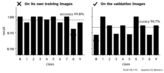
DL01.10.1-F5
Wrong beside right. Scored on the images it was fitted to, the baseline looks better than it is. The bar must be measured where the network will be measured: on the validation images.
“The baseline scores 99 percent, so the bar is 99 percent.”
That is its accuracy on its own training images, which it has partly memorised (ML01.2.1). On images it has not seen it scores 96.7 percent. Compare like with like: the network’s validation accuracy against the baseline’s validation accuracy.
“Accuracy is always the score to use.”
Here it is fair because the classes are balanced, as the formula shows. On a set where one class is 99 percent of the images, the majority rule scores 99 percent and finds none of the rare class (ML01.7.1). Look at the class counts before choosing the score.
“A majority baseline is too silly to bother with.”
It costs one line and it catches broken pipelines. A network whose validation accuracy sits at about 10 percent has learned nothing, and lesson DL01.10.2 meets one.
“Let me check the test images too, to see how hard the task is.”
The test set stays closed until one final measurement (DL01.10.3). Every look at it that changes a decision makes the final number less honest (ML01.9.4).
Check yourself
Recall
1. What are the input, the output and the score of this project?
Show answer
The input is 64 pixel counts from 0 to 16, divided by 16; the output is one of ten classes; the score is accuracy, with the recall of each class reported beside it.
2. Write accuracy in terms of the per-class recalls.
Show answer
\({A = \sum_k (n_k / n)\, R_k}\): the recalls weighted by the class shares.
3. Why does the majority rule predict 1 here, and what does it score on validation?
Show answer
Classes 1, 3, 4, 5 and 6 tie with 109 training images and the first of them, 1, is taken. The validation set holds 37 ones, so it scores \({37/360 = 0.103}\).
4. What validation accuracy does logistic regression reach, and what does that mean for the network?
Show answer
348 of 360, 96.7 percent. The network must beat that to justify its hidden layer.
5. Why is dividing by 16 safe from leakage, when standardising with the mean of all images is not?
Show answer
16 is fixed by how the data were made, not computed from any images, so no information from the validation or test images enters training.
Exercises
1.★ A classifier on the validation set has recall 0.5 on class 2 and recall 1 on every other class. Using the validation counts (35, 37, 36, 37, 36, 36, 36, 36, 35, 36), find its accuracy twice: by counting, and with the weighted formula.
Show solution
Counting: class 2 has 36 images and half of them, 18, are wrong; every other image is right, so 342 of 360 are right and \({A = 342/360}\), which is 0.95. Formula: class 2 has share \({36/360 = 0.1}\) and the other classes together \({324/360 = 0.9}\), so
\[
A = 0.1 \cdot 0.5 + 0.9 \cdot 1 = 0.95 .
\]
The two agree, as they must.
2.★★ Prove that no constant rule (one that always answers the same class) can beat the majority rule on the data it was fitted to, and say why it can still lose on the validation set.
Show solution
A rule that always answers \(m\) has \({R_m = 1}\) and every other recall 0, so its accuracy is \({n_m / n}\). On the training data the majority class has the largest \(n_m\), so no constant rule does better. On the validation set the counts differ: there classes 1 and 3 both have 37 images, the largest count, so answering 3 would also score 37/360, while answering 4, 5 or 6, tied with 1 in training, would score only 36/360. The fitted rule is best on the data it saw, not necessarily on new data.
3.★★★ A set has two classes, 990 images of A and 10 of B. Model P has recalls 1.0 on A and 0.0 on B; model Q has 0.95 and 0.9. Compute both accuracies and both plain means of the recalls, and explain with the formula why they rank the models differently.
The plain means of the recalls are \({(1 + 0)/2 = 0.5}\) for P and \({(0.95 + 0.9)/2 = 0.925}\) for Q. Accuracy prefers P, the plain mean prefers Q. The formula weights each recall by its class share, 0.99 against 0.01, so class B’s recall barely moves the accuracy; the plain mean gives both classes the weight one half. With balanced classes the two weightings agree, which is why accuracy is fair on the digits.
Summary card
Say the task, choose the score, and set the bar before training.
DL01.10.1-F1
Ten classes, 64 pixels, two baselines.
Accuracy is the share-weighted mean of the recalls: \({A = \sum_k (n_k/n) R_k}\).
Constant rule answering \(m\): accuracy \({n_m / n}\); here class 1, \({37/360 = 0.103}\).
Logistic regression on pixels divided by 16: 348 of 360, 96.7 percent on validation.
Balanced classes, so accuracy is fair; report the recalls beside it.
Sources and next steps
Sources. Each was opened and checked against this lesson on 15 November 2026.
scikit-learn 1.9 user guide, Toy datasets, section on the optical recognition of handwritten digits: 1,797 instances, 64 attributes, an 8 by 8 image of integer pixels in the range 0 to 16, made by counting the on pixels in non-overlapping 4 by 4 blocks of 32 by 32 bitmaps; a copy of the test set of the UCI dataset.
scikit-learn 1.9 API reference, DummyClassifier: with strategy="most_frequent", predict always returns the most frequent class label of the y given to fit. The page does not say how a tie is broken; the code above checks it.
scikit-learn 1.9 API reference, LogisticRegression: defaults C=1.0, an L2 penalty and the lbfgs solver; with three or more classes it fits the multinomial (softmax) loss.
scikit-learn 1.9 API reference, classification_report: precision, recall, F1 and support per class, with the macro average (unweighted) and the weighted average (weighted by support).
Next.DL01.10.2 Train the network builds the 64-32-10 network, checks the training loop and picks a width and a learning rate on the validation set.