An artificial neuron takes a weighted sum of its inputs, adds a bias and passes the result through an activation. With the identity it is linear regression; with the sigmoid it is logistic regression. One training loop fits both.
DL01.1.1L2 Intermediate25 minIn review (what this means)
The maths and code on this page are checked by automated tests on every change, but an independent reader has not signed it off yet. Spot a mistake or a confusing step? Tell us.
Write the computation of an artificial neuron, a weighted sum plus a bias followed by an activation, and name each part.
Show that a neuron with the identity activation and the mean squared error is linear regression, and recover the line 1.4x + 0.5.
Show that a neuron with the sigmoid activation and the log loss is logistic regression.
Derive the gradient of either loss with respect to the weighted sum, and train a neuron by gradient descent in NumPy.
Check a NumPy neuron against scikit-learn’s LinearRegression and LogisticRegression.
The question
Every network in this course is built from one small unit, repeated: the digit classifier at the end of DL01 has 42 of them, and a large language model repeats it on a vast scale, with billions of weights. You have already trained two of these units in ML01, under other names. Which two, and what single piece of code trains both?
Intuition
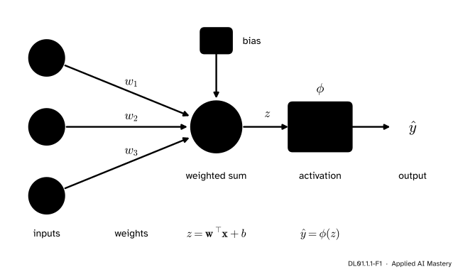
An artificial neuron reads a few numbers, its inputs. It multiplies each input by a weight, adds the products together with one more number, the bias, and passes the total through a fixed function, the activation. What comes out is the neuron’s output.
DL01.1.1-F1
The neuron diagram used through the course. Inputs are blue, the weights and the bias are orange, and everything the neuron computes is vermillion. The weighted sum \(z\) is a line; the activation \(\phi\) bends it.
The name comes from biology. A nerve cell collects signals from other cells through synapses of different strengths and fires when the total is large enough. The artificial neuron keeps only that outline: weighted inputs, a sum, a response. It is a very coarse model of a real neuron, and nothing in this course depends on the biology. What matters is that the unit is simple to compute, simple to differentiate, and powerful when many of them are wired together.
Look at the diagram again. Everything left of the activation is the linear model of ML01.4. The only new part is the box on the right.
Build it up
Step 1. The weighted sum. With \(d\) inputs \(x_1, \dots, x_d\) and weights \(w_1, \dots, w_d\), the neuron first computes
\[
\begin{aligned}
z &= w_1 x_1 + w_2 x_2 + \dots + w_d x_d + b \\
&= \vect{w}\T\vect{x} + b .
\end{aligned}
\]
The number \(z\) is called the pre-activation. It is exactly the score of a linear model.
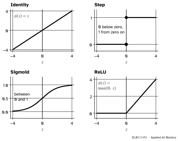
Step 2. The activation. The output is \(\hat{y} = \phi(z)\), where \(\phi\) (the Greek letter phi) is a function of one number. Four choices appear in this module.
DL01.1.1-F2
Four activations. The identity changes nothing, the step answers yes or no, the sigmoid gives a probability, and the ReLU (rectified linear unit) keeps positive values and zeroes the rest.
Step 3. One input, one neuron. With a single input, \(z = wx + b\) is a straight line in \(x\). Choose the identity and the neuron is the line. Choose the sigmoid and the neuron is the S-shaped curve of ML01.6.1.
Step 4. A loss and a training rule. A neuron alone is only a function. To learn its weights we need a loss that scores its outputs against the targets, and gradient descent from ML01.5 to lower that loss. The pair (activation, loss) decides which model you get.
The formal statement
NoteDefinition: an artificial neuron
A neuron with \(d\) inputs has a weight vector \(\cparam{\vect{w}}\) in \(\R^d\), a bias \(\cparam{b}\) and an activation \(\phi\). For an input \(\cdata{\vect{x}}\) in \(\R^d\) it computes
Two choices of activation and loss give models you already know.
Identity and mean squared error: linear regression. With \(\phi(z) = z\) and one input, the neuron outputs \(\hat{y}_i = wx_i + b\), and the mean squared error
\[
L = \frac{1}{n}\sum_{i=1}^{n} (wx_i + b - y_i)^2
\]
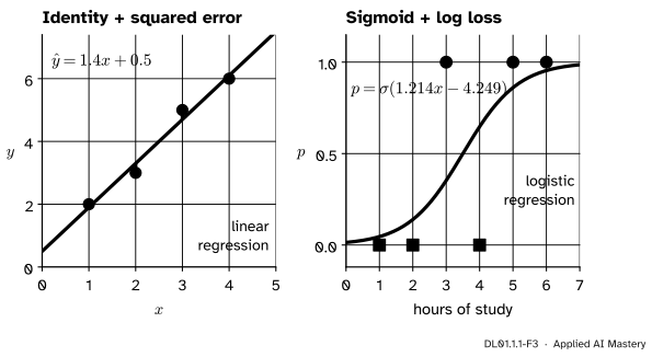
is the loss of ML01.4. On the four points \({x = (1, 2, 3, 4)}\) and \({y = (2, 3, 5, 6)}\) its minimum is at \({w = 1.4}\), \({b = 0.5}\), with \({L = 0.05}\) (ML01.5.1).
Sigmoid and log loss: logistic regression. With \(\phi = \sigma\), the output \({p_i = \sigma(wx_i + b)}\) is read as a probability, and the loss is the mean log loss of ML01.6.2,
On the six students of ML01.6 (hours 1 to 6, passed \(0, 0, 1, 0, 1, 1\)) its minimum is at \({w = 1.214}\), \({b = -4.249}\), with \({L = 0.413}\) (ML01.6.3).
DL01.1.1-F3
One neuron, two activations, two familiar models. Left: the identity neuron fitted by the mean squared error. Right: the sigmoid neuron fitted by the log loss.
The gradient goes through \(z\). Write \(z_i = wx_i + b\) for example \(i\). The loss depends on \(w\) and \(b\) only through the \(z_i\), so by the chain rule
Sigmoid and log loss. Take the loss of one example, \({\ell = -[\,y \ln p + (1 - y)\ln(1 - p)\,]}\), and differentiate in two steps. First with respect to \(p\):
Then \(\frac{dp}{dz} = p(1 - p)\), the derivative of the sigmoid (derived below). The product is
\[
\frac{d\ell}{dz} = \frac{p - y}{p(1 - p)} \cdot p(1 - p) = p - y ,
\]
and with the factor \(\frac{1}{n}\) of the mean, \({\pd{L}{z_i} = \frac{1}{n}(p_i - y_i)}\).
Both models train with one loop. In each case the gradient at the weighted sum is a constant times (prediction minus target): \(\frac{2}{n}\) for linear regression, \(\frac{1}{n}\) for logistic regression. The rest of the gradient, multiplying by \(x_i\) and summing, is the same. That is the code the hook asked for.
Go deeper: the derivative of the sigmoid
Write \({\sigma(z) = (1 + e^{-z})^{-1}}\) and use the chain rule:
The last step uses \({\frac{e^{-z}}{1 + e^{-z}} = 1 - \sigma(z)}\), from ML01.6.1. The derivative is largest at \({z = 0}\), where it equals \(\frac14\). DL01.3.1 returns to this number.
Worked example
One example through each neuron, forward and back to \(z\).
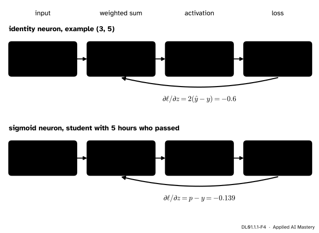
The identity neuron (\({w = 1.4}\), \({b = 0.5}\)) on the point \({(x, y) = (3, 5)}\):
weighted sum: \({z = 1.4 \cdot 3 + 0.5 = 4.7}\);
output: \({\hat{y} = z = 4.7}\);
squared error: \({(4.7 - 5)^2 = 0.09}\);
gradient of this example’s error at \(z\): \({2(\hat{y} - y) = 2 \cdot (-0.3) = -0.6}\).
The sigmoid neuron (\({w = 1.214}\), \({b = -4.249}\)) on the student who studied 5 hours and passed:
gradient at \(z\): \({p - y = 0.861 - 1 = -0.139}\).
DL01.1.1-F4
The worked example as a trace. Forward, left to right; the gradient comes back from the loss to the weighted sum. Both gradients are negative, so gradient descent will raise \(z\) for these examples.
One full gradient step for the identity neuron. Start from \({w = 0}\), \({b = 0}\) with \({\eta = 0.05}\). Every output is \(0\), so \({\pd{L}{z_i} = \frac{2}{4}(0 - y_i) = -0.5\,y_i}\), which is \({(-1, -1.5, -2.5, -3)}\). Then
The update gives \({w = 0 + 0.05 \cdot 23.5 = 1.175}\) and \({b = 0 + 0.05 \cdot 8 = 0.4}\): the first step of ML01.5.2, now read as a neuron.
Code
A neuron is one line of NumPy. Rows of X are examples and columns are inputs, so X @ w + b is the weighted sum of every example at once.
import numpy as npdef identity(z):return zdef sigmoid(z):return1.0/ (1.0+ np.exp(-z))def neuron(X, w, b, phi):"""One neuron on a batch: each row of X is one example."""return phi(X @ w + b)x_four = np.array([[1.0], [2.0], [3.0], [4.0]]) # one input, as a columny_four = np.array([2.0, 3.0, 5.0, 6.0])hours = np.array([[1.0], [2.0], [3.0], [4.0], [5.0], [6.0]])passed = np.array([0.0, 0.0, 1.0, 0.0, 1.0, 1.0])print("identity neuron at x = 3:", neuron(np.array([[3.0]]), np.array([1.4]), 0.5, identity))print("sigmoid neuron at 5 hours:", neuron(np.array([[5.0]]), np.array([1.214]), -4.249, sigmoid).round(3))
identity neuron at x = 3: [4.7]
sigmoid neuron at 5 hours: [0.861]
Training needs only the gradient at \(z\), a constant times (prediction minus target). One function serves both models; the argument scale is \(\frac{2}{n}\) or \(\frac{1}{n}\).
def train(X, y, phi, scale, lr, steps):"""Gradient descent on one neuron, starting from zero. dL/dz_i = scale * (yhat_i - y_i).""" w, b = np.zeros(X.shape[1]), 0.0for _ inrange(steps): g = scale * (neuron(X, w, b, phi) - y) # dL/dz, one entry per example w = w - lr * (X.T @ g) # dL/dw = sum of g_i x_i b = b - lr * g.sum() # dL/db = sum of g_ireturn w, bw_one, b_one = train(x_four, y_four, identity, scale=2/4, lr=0.05, steps=1)print(f"after one step: w = {w_one[0]:.4f}, b = {b_one:.4f}")w_lin, b_lin = train(x_four, y_four, identity, scale=2/4, lr=0.05, steps=5000)w_log, b_log = train(hours, passed, sigmoid, scale=1/6, lr=0.3, steps=3000)print(f"linear neuron: w = {w_lin[0]:.4f}, b = {b_lin:.4f}")print(f"logistic neuron: w = {w_log[0]:.4f}, b = {b_log:.4f}")
after one step:  w = 1.1750, b = 0.4000
linear neuron:   w = 1.4000, b = 0.5000
logistic neuron: w = 1.2140, b = -4.2491
The derivation of \(\pd{L}{z_i}\) can be checked without trusting it: nudge \(w\) a little each way and measure how the log loss moves (a central difference, as in ML01.6.3).
Last, the library. scikit-learn’s LinearRegression minimises the squared error exactly. LogisticRegression adds a penalty on the weights unless it is told not to; C=np.inf switches it off, which is how scikit-learn 1.9 asks for the plain log loss.
from sklearn.linear_model import LinearRegression, LogisticRegressionlin = LinearRegression().fit(x_four, y_four)log = LogisticRegression(C=np.inf).fit(hours, passed)print(f"LinearRegression: w = {lin.coef_[0]:.4f}, b = {lin.intercept_:.4f}")print(f"LogisticRegression: w = {log.coef_[0, 0]:.4f}, b = {log.intercept_[0]:.4f}")
LinearRegression:   w = 1.4000, b = 0.5000
LogisticRegression: w = 1.2141, b = -4.2493
The four numbers agree with the hand-written neuron, the logistic ones to three decimals: the two programs stop their searches at slightly different places.
Explore
The module’s interactive, the neuron playground, is in lesson 2. It is a neuron with two inputs: move \(w_1\), \(w_2\) and \(b\), switch the activation between step, sigmoid and ReLU, and watch the plane change colour while the line \({z = 0}\) stays exactly where it is.
Pitfalls
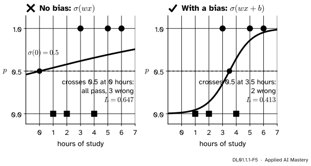
DL01.1.1-F5
Wrong beside right. Left: the best sigmoid neuron without a bias must give \(0.5\) at zero hours, so it calls every student a pass. Right: the bias moves the midpoint to \(3.5\) hours.
“The bias is a detail; the weights do the work.”
Without a bias, \(z = wx\) is \(0\) at \({x = 0}\), so the sigmoid neuron must output \(0.5\) there and its boundary is pinned to the origin. The best it can do on the six students is \({w = 0.162}\) with a log loss of \(0.647\), calling all six a pass. The bias is what lets the boundary sit anywhere.
“A sigmoid output trained with squared error is still logistic regression.”
The model is the neuron and its loss. The same sigmoid neuron trained with the squared error is a different model with a different gradient, \({\frac{2}{n}(p - y)\,p(1 - p)}\), which almost vanishes when the neuron is confidently wrong. DL01.4.2 shows why the log loss is the right partner.
“An artificial neuron works like a brain cell.”
It borrows a picture, nothing more. Real neurons send spikes in time, adapt and are wired in ways this sum-and-squash unit ignores. Judge the unit by what it computes, not by its name.
Check yourself
Recall
1. Write the two steps a neuron computes, and name \(z\).
Show answer
\({z = \vect{w}\T\vect{x} + b}\), the pre-activation (the weighted sum plus the bias), then \({\hat{y} = \phi(z)}\).
2. Which activation and loss make a neuron into linear regression, and which into logistic regression?
Show answer
The identity with the mean squared error gives linear regression; the sigmoid with the log loss gives logistic regression.
3. What is \({\pd{L}{z_i}}\) for a sigmoid neuron with the mean log loss over \(n\) examples?
Show answer
\(\frac{1}{n}(p_i - y_i)\): prediction minus target, divided by \(n\).
4. Given \({\pd{L}{z_i}}\) for every example, how do you get \({\pd{L}{w}}\) and \({\pd{L}{b}}\) for a neuron with one input?
Show answer
Multiply each \({\pd{L}{z_i}}\) by \(x_i\) and add them for \({\pd{L}{w}}\); add them as they are for \({\pd{L}{b}}\).
5. What does the bias let a neuron do that the weights alone cannot?
Show answer
Move its boundary \({z = 0}\) away from the origin. Without a bias, \({z = 0}\) whenever \({\vect{x} = \vect{0}}\).
Exercises
1.★ A neuron has \({\vect{w} = (2, -1)}\) and \({b = 0.5}\). For \({\vect{x} = (1, 3)}\), find \(z\) and the output with each of the four activations of this lesson.
2.★★ The identity neuron on the four points sits at \({w = 1}\), \({b = 0}\). Compute \({\pd{L}{z_i}}\) for each point, then \(\pd{L}{w}\) and \(\pd{L}{b}\), and take one step with \({\eta = 0.05}\).
Show solution
The outputs are \({(1, 2, 3, 4)}\), so the errors and the gradients at \(z\) are
One step: \({w = 1 + 0.05 \cdot 8.5 = 1.425}\) and \({b = 0 + 0.05 \cdot 3 = 0.15}\), as in ML01.5.2.
3.★★★ At the minimum of the mean log loss both partial derivatives are zero. Show that the fitted sigmoid neuron’s probabilities then add up to the number of passes, and that \({\sum_i p_i x_i = \sum_i y_i x_i}\). Check both on the six students.
Show solution
From \({\pd{L}{b} = \frac{1}{n}\sum_i (p_i - y_i) = 0}\) we get \({\sum_i p_i = \sum_i y_i}\), the number of passes. From \({\pd{L}{w} = \frac{1}{n}\sum_i (p_i - y_i)\,x_i = 0}\) we get \({\sum_i p_i x_i = \sum_i y_i x_i}\).
On the six students three passed, so the six probabilities of the fitted neuron add up to \(3\). The students who passed studied 3, 5 and 6 hours, so \({\sum_i p_i x_i = 3 + 5 + 6 = 14}\). The lesson’s code confirms both to five decimals. (The same argument for the identity neuron shows that its residuals add up to zero.)
Summary card
A neuron is a weighted sum, a bias and an activation.
Linear regression. Identity and mean squared error: \({\hat{y} = 1.4x + 0.5}\) on the four points.
Logistic regression. Sigmoid and log loss: \({w = 1.214}\), \({b = -4.249}\) on the six students.
Gradient at \(z\).\(\frac{2}{n}(\hat{y}_i - y_i)\) or \(\frac{1}{n}(p_i - y_i)\); then multiply by \(x_i\) and sum.
Sources and next steps
Sources. Each was opened and checked against this lesson on 15 November 2026.
Stanford CS231n, Neural Networks Part 1: Setting up the Architecture, section “Modeling one neuron”. Each neuron “performs a dot product with the input and its weights, adds the bias and applies the non-linearity”; the section on a single neuron as a linear classifier shows that one neuron trained with the right loss is a binary Softmax (logistic) classifier; and the notes call this model of a biological neuron “very coarse”.
Simon J. D. Prince, Understanding Deep Learning (MIT Press, 2023, free PDF). Section 3.5 names the values before the activation pre-activations and those after it activations, and notes that hidden units are sometimes called neurons.
Ian Goodfellow, Yoshua Bengio and Aaron Courville, Deep Learning, Section 6.1: most neural networks apply “an affine transformation controlled by learned parameters, followed by a fixed nonlinear function called an activation function”.
scikit-learn 1.9.1 documentation, LinearRegression (ordinary least squares) and LogisticRegression, where C=np.inf “results in unpenalized logistic regression” and the penalty argument is deprecated since version 1.8.