A classifier can learn the border between classes directly, or learn what each class looks like and let Bayes’ rule do the rest. See both routes on one feature, prove that the largest posterior gives the lowest error rate, and find the best threshold by hand.
ML02.6.1L2 Intermediate25 minIn review (what this means)
The maths and code on this page are checked by automated tests on every change, but an independent reader has not signed it off yet. Spot a mistake or a confusing step? Tell us.
Distinguish a generative classifier, which models p(x | y) and p(y), from a discriminative one, which models p(y | x) directly.
Turn class-conditional densities and priors into a posterior with Bayes’ rule, and classify by the largest posterior.
Prove that the Bayes classifier has the lowest possible error rate for two classes by comparing the two weighted densities point by point.
Find the decision threshold of two Gaussian classes with equal spread, by hand and from data.
The question
Logistic regression learned where “pass” turns into “fail” and nothing else. There is a second way to build a classifier: learn what each class looks like, then ask which class would most plausibly have produced the new example. Which way is right, and is there a best possible classifier that both are trying to reach?
Intuition
Take one feature \(x\) and two classes, 0 and 1. A discriminative classifier models the answer we want, the probability of each class given \(x\), and nothing more. Logistic regression (ML01.6) is the standard example: it fits an S-shaped curve for \({p(y = 1 \mid x)}\) straight to the labels.
A generative classifier models how the data are made. It describes the values of \(x\) that each class tends to produce, \({p(x \mid k)}\), and how common each class is, \(\pi_k\). Then it turns these around with Bayes’ rule (M06.4) to get the probability of each class given \(x\).
ML02.6.1-F1
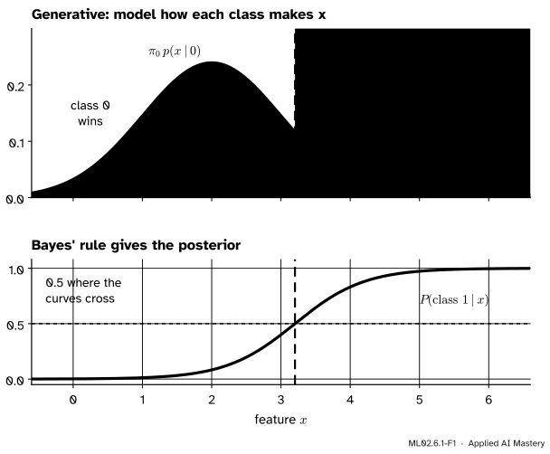
The generative route for two classes. Class 0 makes values near 2 and is more common (prior 0.6); class 1 makes values near 4 (prior 0.4). Where the weighted curves cross, the posterior is exactly 0.5, and that point is the decision threshold.
Read the top panel as two stories. “Class 0 happens 60% of the time and its \(x\) is usually near 2.” “Class 1 happens 40% of the time and its \(x\) is usually near 4.” For a new \(x\), compare the heights of the two curves there. The taller one is the more plausible source, so it wins. The bottom panel is the same comparison written as a probability.
Build it up
Step 1. One density per class. The class-conditional density\({p(x \mid k)}\) says where the values of \(x\) fall when the class is \(k\). It is a density over \(x\) (M06.6), so it has area 1 for each class. Here both classes are bells of spread \({\sigma = 1}\): class 0 is centred at \({\mu_0 = 2}\) and class 1 at \({\mu_1 = 4}\).
Step 2. One prior per class. The prior\(\pi_k\) is the share of class \(k\) before any \(x\) is seen: \({\pi_0 = 0.6}\) and \({\pi_1 = 0.4}\). The product \({\pi_k\, p(x \mid k)}\) is the joint density of “class \(k\) and value \(x\)”. The curves in the top panel of the anchor figure are these products, so class 1’s bell is lower than class 0’s.
Step 3. Bayes’ rule. Divide each product by their sum to get the posterior:
The denominator is \({p(x)}\), the same for both classes, so it only rescales. Which class is larger is already settled by the products.
Step 4. Decide. Predict the class with the larger posterior. With two classes that means class 1 exactly when \({p(1 \mid x) \ge 0.5}\), which happens where the weighted curves cross.
ML02.6.1-F2
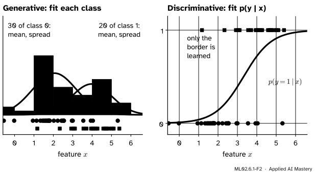
Two routes from the same data. The generative route fits a mean, a spread and a share for each class. The discriminative route fits the S-curve to the labels and never says what a typical \(x\) of either class looks like.
The two routes differ in what they learn. The generative model can also say how likely a value of \(x\) is at all, and could even draw new examples. The discriminative model spends all its effort on the border, which is all that classification needs.
The formal statement
NoteDefinitions
A discriminative classifier models \({p(y \mid \vect{x})}\) directly. A generative classifier models \({p(\vect{x} \mid y = k)}\) and the priors \({\pi_k = \Prob(y = k)}\), and computes \({p(y = k \mid \vect{x})}\) from them by Bayes’ rule.
The Bayes classifier predicts the class with the largest posterior, \({\argmax_k \pi_k\, p(\vect{x} \mid k)}\). Its error rate is the Bayes error rate.
NoteTheorem: the Bayes classifier has the lowest error rate
If the densities and priors are the true ones, no classifier has a lower expected error rate than the Bayes classifier.
Proof for two classes and one feature. Any classifier splits the line into a region \(R_1\) where it predicts class 1 and a region \(R_0\) where it predicts class 0. It errs on a class-0 example that lands in \(R_1\), and on a class-1 example that lands in \(R_0\). Adding the two kinds of mistake,
Every point \(x\) lies in exactly one region, so it adds exactly one of its two heights to the error: \({\pi_0\, p(x \mid 0)}\) if it is in \(R_1\), or \({\pi_1\, p(x \mid 1)}\) if it is in \(R_0\). Whatever the classifier does at \(x\), it adds at least the smaller of the two. So
The Bayes classifier puts each \(x\) in the region of the larger height, so it adds exactly the smaller one at every point and meets this bound. No classifier can do better. \(\square\)
ML02.6.1-F3
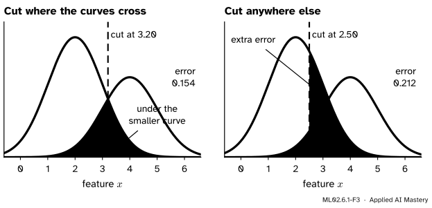
The proof as a picture. The error is the area that the classifier leaves under the curve of the class it did not pick. Cutting where the curves cross leaves only the smaller curve. Moving the cut adds a sliver between the curves.
Two remarks. First, the Bayes error rate is not zero when the classes overlap: here it is 0.154, a floor that no model can go below, however much data it has. Second, real classifiers never know the true densities. A generative classifier estimates them and plugs the estimates into Bayes’ rule, so it is only as good as its model of each class.
The posterior is a logistic curve. For two Gaussian classes with the same spread \(\sigma\), take the log of the ratio of the two products. The factors \({1/(\sigma\sqrt{2\pi})}\) cancel, so
So \({p(1 \mid x) = \sigma(wx + b)}\), the very form of logistic regression. The two models share a shape and differ in how they choose \(w\) and \(b\): logistic regression picks them to fit the labels, the generative model computes them from means, a spread and priors. (Here \(\sigma\) inside the brackets is the sigmoid of ML01.6, not the spread.)
Go deeper: many classes, and why the denominator never matters
With \(K\) classes the posterior is \({\pi_k\, p(x \mid k) / \sum_j \pi_j\, p(x \mid j)}\). The denominator is the same for every \(k\), so the class with the largest posterior is the class with the largest product \({\pi_k\, p(x \mid k)}\), and taking logs does not change which is largest. The proof above carries over: the probability of a correct answer is \({\int \pi_{h(x)}\, p(x \mid h(x))\,dx}\) for a classifier \(h\), and at each \(x\) the integrand is at most \({\max_k \pi_k\, p(x \mid k)}\), which the Bayes classifier reaches.
Worked example
Classes 0 and 1 have bells \({N(2, 1)}\) and \({N(4, 1)}\), with priors 0.6 and 0.4. Where is the threshold, and what is the posterior at \({x = 3}\)?
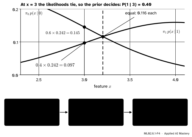
At \({x = 3}\). The point is one unit from both means, so both densities are \({\tfrac{1}{\sqrt{2\pi}}e^{-1/2} = 0.242}\). The products are \({0.6 \times 0.242 = 0.145}\) and \({0.4 \times 0.242 = 0.097}\). Their sum is 0.242, so
\[
p(1 \mid 3) = \frac{0.097}{0.242} = 0.40 .
\]
When the likelihoods tie, the evidence says nothing and the posterior equals the prior.
ML02.6.1-F4
The worked example. At \({x = 3}\) the prior tips the balance to class 0. The weighted curves meet a little further right, at 3.203, where both heights are 0.116.
The threshold. Set the two log products equal. The common factor \({1/\sqrt{2\pi}}\) cancels:
and the right side is \({2\ln(2/3) = -0.811}\). So \({4x = 12.811}\) and
\[
x = 3 + \tfrac{1}{2}\ln 1.5 = 3.203 .
\]
Without priors the cut would sit halfway, at 3. The rarer class 1 has to earn its prediction, so the cut moves 0.203 towards it. The formula from the formal section agrees: \({w = 2/1 = 2}\) and \({b = (4 - 16)/2 + \ln(2/3) = -6.405}\), so the posterior is \({\sigma(2x - 6.405)}\), which is 0.5 at \({x = 6.405/2 = 3.203}\).
The error. With the cut at 3.203, a class-0 example errs when its value lands above the cut, and a class-1 example when it lands below:
A cut at 3 gives 0.159, and a cut at 2.5 gives 0.212.
Code
First the exact answers, then a generative classifier fitted to data, from scratch.
import mathimport numpy as npdef Phi(z):"""The standard normal cumulative distribution."""return0.5* (1+ math.erf(z / math.sqrt(2)))def error(cut, pi1=0.4, mu0=2.0, mu1=4.0):"""Error of 'class 1 when x >= cut' for the two bells of spread 1."""return (1- pi1) * (1- Phi(cut - mu0)) + pi1 * Phi(cut - mu1)c_exact =3+0.5* math.log(1.5)print(f"threshold {c_exact:.4f}, Bayes error {error(c_exact):.4f}")print(f"cut at 3: {error(3):.4f} cut at 2.5: {error(2.5):.4f}")
threshold 3.2027, Bayes error 0.1538
cut at 3: 0.1587   cut at 2.5: 0.2118
Now draw 2,000 labelled examples and fit the generative model: the share of each class, the two means, and one shared spread (the average squared distance of each point from its own class mean).
prior 0.407, means 1.996 and 4.000, variance 0.994
generative threshold 3.183
The discriminative route on the same data is logistic regression. A huge C switches off its penalty, so it fits the labels as they are.
from sklearn.linear_model import LogisticRegressionlr = LogisticRegression(C=1e6).fit(x[:, None], y)w, b = lr.coef_[0, 0], lr.intercept_[0]print(f"logistic regression: w = {w:.3f}, b = {b:.3f}, threshold {-b / w:.3f}")
logistic regression: w = 1.959, b = -6.265, threshold 3.199
Both routes land within a few hundredths of 3.203, and logistic regression’s weight is near the \({w = 2}\) that the formula predicts. With the right model of each class and plenty of data, the two routes agree. They part ways when the class model is wrong or the data are few, which is the story of lesson ML02.6.4.
Explore
This module’s interactive, the two-class Gaussian explorer, sits in lesson ML02.6.4. You can use it now: drag the two means, change the spreads and slide the prior, and watch the threshold and the shaded Bayes error move. Give the classes different spreads and a second threshold appears. Leave the “duplicate the feature” button alone until that lesson.
Pitfalls
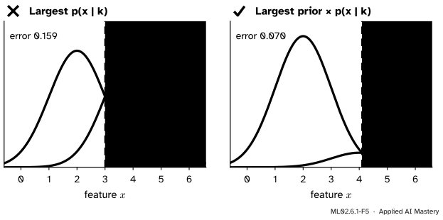
ML02.6.1-F5
Wrong beside right, with a rare class 1 (prior 0.1). Comparing likelihoods alone puts the cut at 3 and errs 15.9% of the time. Weighting by the priors moves it to 4.10 and more than halves the error.
“The class that makes this \(x\) most likely is the most likely class.”
That compares \({p(x \mid k)}\), the likelihood, when the decision needs \({p(k \mid x)}\), the posterior. They differ by the prior. With a rare class, as in the figure, ignoring the prior predicts it far too often. A fraud detector or a screening test that does this raises a flood of false alarms.
“The Bayes classifier is perfect.”
It is the best possible, which is not the same thing. Where the classes overlap, some examples of class 1 look exactly like typical examples of class 0, and no rule can tell them apart. Here the floor is 15.4%. A model that claims much less on new data is being tested on the wrong data.
“Discriminative models always win, because they model what we care about.”
They have the lower error when data are plentiful, but a generative model can reach its best error with far fewer examples. Ng and Jordan found both regimes on real datasets, as lesson ML02.6.4 shows.
Check yourself
Recall
1. What does a generative classifier model, and what does a discriminative one model?
Show answer
A generative classifier models \({p(\vect{x} \mid y)}\) for each class and the priors \({\Prob(y)}\), then uses Bayes’ rule. A discriminative classifier models \({p(y \mid \vect{x})}\) directly.
2. State the Bayes classifier.
Show answer
Predict the class \(k\) with the largest posterior \({p(k \mid \vect{x})}\), which is the class with the largest product \({\pi_k\, p(\vect{x} \mid k)}\).
3. In the proof that it is optimal, what does each point \(x\) add to the error rate?
Show answer
One of its two weighted heights: \({\pi_0\, p(x \mid 0)}\) if it is classed as 1, or \({\pi_1\, p(x \mid 1)}\) if it is classed as 0. The Bayes classifier always adds the smaller one.
4. For two Gaussian classes with the same spread, what shape does the posterior \({p(1 \mid x)}\) have?
Show answer
A logistic curve \({\sigma(wx + b)}\) with \({w = (\mu_1 - \mu_0)/\sigma^2}\), the same form as logistic regression.
5. In the worked example, why is the threshold 3.203 and not 3?
Show answer
Class 1 is the rarer class (prior 0.4), so its curve is scaled down and meets class 0’s curve to the right of the midpoint, by \({\tfrac12 \ln 1.5 = 0.203}\).
Exercises
1.★ Keep the bells \({N(2, 1)}\) and \({N(4, 1)}\). Find the threshold when the priors are equal, and when class 1 has prior 0.2.
Show solution
The general threshold for equal spread 1 (exercise 3) is
Equal priors give \({\ln 1 = 0}\), so the cut is at 3. With \({\pi_1 = 0.2}\) the cut is \({3 + \tfrac12 \ln(0.8/0.2)}\)\({= 3 + \tfrac12 \ln 4}\)\({= 3.693}\).
2.★★ Class 0 is \({N(0, 1)}\) and class 1 is \({N(0, 4)}\), a bell with spread 2, and the priors are equal. Where does the Bayes classifier predict class 1?
Show solution
Compare the log densities. Class 0 gives \({-\ln\sqrt{2\pi} - x^2/2}\); class 1 gives \({-\ln\sqrt{2\pi} - \ln 2 - x^2/8}\). Class 1 wins when
\[
-\frac{x^2}{8} - \ln 2 > -\frac{x^2}{2} ,
\]
that is \({\tfrac38 x^2 > \ln 2}\), so \({x^2 > \tfrac83 \ln 2 = 1.848}\) and \({\abs{x} > 1.360}\). The wide class wins in both tails, so there are two thresholds. With unequal spreads the \(x^2\) terms do not cancel, and the boundary is no longer a single cut.
3.★★★ Show that for two Gaussian classes with equal spread the threshold always moves away from the midpoint towards the rarer class, by \({\sigma^2 \ln(\pi_0/\pi_1)/(\mu_1 - \mu_0)}\) when \({\mu_0 < \mu_1}\).
Show solution
The threshold is where the log-odds \({wx + b}\) are zero, so \({x = -b/w}\). With the \(w\) and \(b\) of the formal section,
The first step divides each term of \(b\) by \(w\); the second uses \({\mu_1^2 - \mu_0^2 = (\mu_1 - \mu_0)(\mu_1 + \mu_0)}\) and \({-\ln(a/b) = \ln(b/a)}\). If class 1 is rarer, \({\pi_0 > \pi_1}\), the shift is positive: the cut moves right, towards class 1’s mean. If class 0 is rarer the shift is negative and the cut moves towards \(\mu_0\).
Summary card
Model each class, weight it by its prior, and the larger curve decides.
ML02.6.1-F1
Weighted curves cross where the posterior is 0.5.
Generative: model \({p(\vect{x} \mid k)}\) and \(\pi_k\), then \({p(k \mid \vect{x}) \propto \pi_k\, p(\vect{x} \mid k)}\).
Discriminative: model \({p(y \mid \vect{x})}\) directly, as logistic regression does.
Bayes classifier:\({\argmax_k \pi_k\, p(\vect{x} \mid k)}\), the lowest possible error rate.
Equal-spread Gaussians: the threshold is the midpoint of the means, moved towards the rarer class by \({\tfrac{\sigma^2}{\mu_1 - \mu_0}\ln\tfrac{\pi_0}{\pi_1}}\).
Sources and next steps
Sources. Each was opened and checked against this lesson on 15 November 2026.
G. James, D. Witten, T. Hastie and R. Tibshirani, An Introduction to Statistical Learning, 2nd edition (free PDF). Section 4.4 introduces generative models for classification: model the predictors in each class, flip them with Bayes’ theorem (equation 4.15), and approximate the Bayes classifier, which has the lowest possible error rate. Section 4.4.1 gives the one-predictor Gaussian case and the midpoint boundary (4.19) for equal priors.
A. Y. Ng and M. I. Jordan, On Discriminative vs. Generative Classifiers, NIPS 14 (2001). The abstract states the two regimes: discriminative learning has the lower asymptotic error, while a generative classifier may approach its higher one much faster.