Categorical features without leakage: CatBoost’s ideas
Replacing a category by the mean label of its rows looks like a gift and is a trap: each row’s own label leaks into its feature. See the leak on a seeded table, then fix it with CatBoost’s ordered target statistics, cross-fitting, and native categorical splits.
ML02.5.3L2 Intermediate30 minIn review (what this means)
The maths and code on this page are checked by automated tests on every change, but an independent reader has not signed it off yet. Spot a mistake or a confusing step? Tell us.
Encode a categorical column one-hot, ordinally and by its smoothed target mean, and say when each fits.
Derive why the greedy target encoding of a training row depends on its own label, and show the resulting gap between training and test rows.
Compute ordered target statistics along a random permutation, with a prior, by hand and in NumPy.
Use TargetEncoder and native categorical splits in HistGradientBoosting, and describe ordered boosting and oblivious trees.
The question
A column holds a customer id with a thousand values. One-hot coding would add a thousand columns. A neater idea is to replace each id by the share of its rows with label 1. On the training rows that new feature is the best one in the table; on new rows it is worthless. Where does its power come from, and how do you keep the good part?
From the last lesson
1. Why is the gain at a bin edge exact, even though the values were binned?
Show answer
The cut sends exactly the rows of the bins on its left to the left child, and their gradients and Hessians add up bin by bin to the same \(G_L\) and \(H_L\).
2. How does a split decide where rows with a missing value go?
Show answer
It computes the gain with the missing rows’ sums on the left and on the right, and keeps the side with the larger gain as the default direction.
Intuition
A target encoding replaces each category by an estimate of the mean label of its rows. The trouble is in the word its. A customer with two rows in the training data is encoded from those two labels, and one of them is the row’s own label. The feature holds part of the answer.
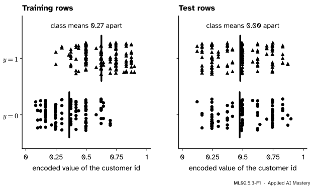
ML02.5.3-F1
The customer id carries no information about the label, by construction. Left: on the training rows its naive target encoding still separates the classes, because each row’s own label is inside its encoding. Right: on test rows the same encoding is noise.
A model trained on the left panel learns “large encoding means label 1”, and is fooled on the right panel. Prokhorenkova and co-authors call this target leakage, and the mismatch between the feature’s behaviour on training and on test rows a conditional shift. The cure is simple to say: never let a row’s own label into its own encoding.
Build it up
Step 1. Three encodings. Take a tiny column of eight colours with labels.
ML02.5.3-F2
Three encodings of one column. One-hot adds a column per category. Ordinal gives each an arbitrary number. Target encoding gives each a smoothed share of label 1, and is the only one that reads the labels.
One-hot is honest and fine for a handful of categories, but adds one column per category. Ordinal codes are compact, but their order is arbitrary, so a tree needs many cuts to group categories that belong together. Target encoding gives one numeric column whose order is the order that matters.
Step 2. Smooth with a prior. A category seen once would get the label of its single row. Mix in a prior \(p\), usually the overall share of label 1, with weight \(a\): the category’s count of label-1 rows plus \(a p\), divided by its number of rows plus \(a\). With \(a = 1\) and \(p = 0.5\), red has rows labelled 1, 1, 0 and gets \({(2 + 0.5)/(3 + 1)} = 0.625\).
Step 3. Leave the row out? A natural repair is leave-one-out: encode each row from the other rows of its category. It fails. Within red, the two rows with \(y = 1\) get \({(1 + 0.5)/3} = 0.5\) and the row with \(y = 0\) gets \({(2 + 0.5)/3} = 0.83\). Inside one category the encoding goes down exactly when the row’s label is 1, so a threshold reads the label off.
Step 4. Use only the past. CatBoost’s ordered target statistic shuffles the rows once into a random order and encodes each row from the rows of its category that come before it. A row’s own label never enters, and neither does any total that contains it.
Step 5. Split on categories directly. LightGBM and scikit-learn can also split a categorical feature without encoding it: sort its categories by a statistic of the gradients in the node, then cut the sorted list like a number line.
The formal statement
NoteDefinition: target statistics
For a training row \(i\) whose category \(c_i\) occurs in a set of rows \(D_i\), with prior \(p\) and weight \(a > 0\),
Greedy:\(D_i\) is every training row. Leave-one-out: every row but \(i\). Ordered: the rows before \(i\) in a random permutation \(\sigma\), that is \({\{ j : \sigma(j) < \sigma(i) \}}\). A test row always uses every training row.
The greedy encoding leaks. Suppose the category says nothing about the label: the labels are independent draws with the same chance of being 1 in every category. Take a training row \(i\) in a category with \(n_c\) training rows, and split the category’s label sum into the row’s own label and the sum \(S\) of the other \(n_c - 1\) labels:
A test row’s encoding is built from training labels only, so its own label does not enter and the same difference is \(0\). The feature behaves differently on the two kinds of rows, which is the conditional shift. The gap is largest for rare categories. With unique categories (\(n_c = 1\)) the paper’s extreme example follows: every training row is encoded \({(y_i + ap)/(1 + a)}\), which takes one value for each label, while every test row gets \(p\).
The ordered encoding does not. Its sum runs over rows \(j\) with \({\sigma(j)} < {\sigma(i)}\), which never includes \(i\). So \(\hat{x}_i\) is a function of other rows’ labels only, and under the same assumption the difference above is \(0\) for training rows as for test rows: the property the paper calls P1. Every row is still used, both to encode later rows and to train the model.
One permutation is noisy. The first rows of the order are encoded from little history, so their values vary a lot. CatBoost draws several permutations and uses a different one at different boosting steps (Section 3.2 and Section 5 of the paper).
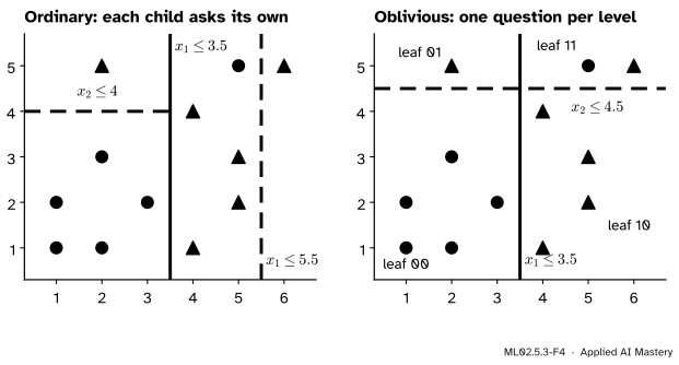
ML02.5.3-F4
Two trees of depth 2 on the course’s twelve points. Left: an ordinary tree asks a different question in each child. Right: an oblivious tree asks the same question across a whole level, so its cuts run across the plane and the \(d\) yes-or-no answers form the leaf’s number.
Ordered boosting and oblivious trees. The same leak recurs in boosting itself: the residual of a training row is computed by a model that was fitted to that very row, so it does not behave like the residual of a new row. The paper calls this prediction shift (Section 4.1). Its ordered boosting (Section 4.2) computes the residual of row \(i\) with a model trained only on the rows before \(i\) in the permutation, and Section 5 shows how to do this without fitting \(n\) models. CatBoost’s trees are oblivious: every node of a level uses the same split. They are balanced, less prone to overfit, and fast to evaluate: a tree of depth \(d\) has \(2^d\) leaves, and the \(d\) answers, read as a binary number, are the leaf’s index.
Go deeper: native categorical splits: why sorting is enough
For a categorical feature with \(K\) categories there are \(2^{K - 1} - 1\) ways to divide them into two groups. scikit-learn sorts the categories by a statistic of the target in each one and considers only the \(K - 1\) cuts of the sorted list, citing Fisher (1958) for why, for the squared loss, the best grouping is always one of these. LightGBM sorts the categories by their accumulated gradient statistics in the node. In scikit-learn the number of categories must stay below max_bins, so a thousand customer ids cannot be split this way.
Worked example
The eight rows of Step 1, in the order shown, which we take as the random order \(\sigma\). The prior is \(p = 0.5\) (four of the eight labels are 1) and \(a = 1\).
Greedy. Red has labels \(1, 1, 0\): \({(2 + 0.5)/4} = 0.625\). Blue has \(0, 1, 0\): \({(1 + 0.5)/4} = 0.375\). Green has \(0, 1\): \({(1 + 0.5)/3} = 0.5\).
Ordered, row by row.
Row
Colour, \(y\)
Before it
Encoding
1
red, 1
none
\(0.5/1 = 0.50\)
2
blue, 0
none
\(0.5/1 = 0.50\)
3
red, 1
red: 1
\(1.5/2 = 0.75\)
4
green, 0
none
\(0.5/1 = 0.50\)
5
blue, 1
blue: 0
\(0.5/2 = 0.25\)
6
red, 0
red: 1, 1
\(2.5/3 = 0.83\)
7
green, 1
green: 0
\(0.5/2 = 0.25\)
8
blue, 0
blue: 0, 1
\(1.5/3 = 0.50\)
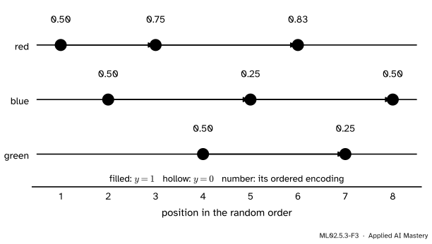
ML02.5.3-F3
The trace of the ordered encoding. Each row is encoded from the rows to its left in its own lane. Row 6 sees two red rows with label 1 and gets \(0.83\), though its own label is 0.
Look at the labels against the encodings. Ordered: the rows with \(y = 1\) got \(0.50\), \(0.75\), \(0.25\) and \(0.25\); those with \(y = 0\) got \(0.50\), \(0.50\), \(0.83\) and \(0.50\). No threshold separates them. Leave-one-out gave every red row with \(y = 1\) the value \(0.5\) and the red row with \(y = 0\) the value \(0.83\), and the same pattern in blue and green: the label, read backwards.
Code
First the three statistics on the eight rows, from scratch.
import numpy as npcolour = np.array(["red", "blue", "red", "green", "blue", "red", "green", "blue"])y8 = np.array([1, 0, 1, 0, 1, 0, 1, 0])prior, a = y8.mean(), 1.0def greedy(cat, y):return np.array([(y[cat == c].sum() + a * prior) / ((cat == c).sum() + a) for c in cat])def leave_one_out(cat, y):return np.array([(y[cat == c].sum() - y[i] + a * prior) / ((cat == c).sum() -1+ a)for i, c inenumerate(cat)])def ordered(cat, y, order): out, total, count = np.empty(len(cat)), {}, {}for i in order: # walk the rows in the random order out[i] = (total.get(cat[i], 0) + a * prior) / (count.get(cat[i], 0) + a) total[cat[i]] = total.get(cat[i], 0) + y[i] count[cat[i]] = count.get(cat[i], 0) +1return outprint("greedy ", greedy(colour, y8).round(3))print("leave-one-out", leave_one_out(colour, y8).round(3))print("ordered ", ordered(colour, y8, range(8)).round(3))
Now the seeded table: a number that matters, one of eight cities with its own effect, and one of a thousand customer ids drawn at random. The first 2,000 rows train, the other 2,000 test.
import osos.environ.setdefault("OMP_NUM_THREADS", "1") # one thread is faster on data this smallfrom sklearn.ensemble import HistGradientBoostingClassifierrng = np.random.default_rng(0)n =4000num = rng.normal(size=n)city = rng.integers(0, 8, size=n)effect = np.array([0.5, -1.5, 1.0, 0.0, 1.5, -1.0, -0.5, 0.0])customer = rng.integers(0, 1000, size=n) # unrelated to the labely = (rng.random(n) <1/ (1+ np.exp(-(num + effect[city])))).astype(int)tr, te =slice(0, 2000), slice(2000, 4000)p = y[tr].mean()total = np.bincount(customer[tr], weights=y[tr], minlength=1000)count = np.bincount(customer[tr], minlength=1000)naive_tr = (total[customer[tr]] + p) / (count[customer[tr]] +1) # a = 1naive_te = (total[customer[te]] + p) / (count[customer[te]] +1)print(f"correlation with the label: training {np.corrcoef(naive_tr, y[tr])[0, 1]:.2f}, "f"test {np.corrcoef(naive_te, y[te])[0, 1]:.2f}")def fit_and_score(extra_tr, extra_te): base_tr = np.c_[num[tr], np.eye(8)[city[tr]]] # the number, and the city one-hot base_te = np.c_[num[te], np.eye(8)[city[te]]] X_tr = base_tr if extra_tr isNoneelse np.c_[base_tr, extra_tr] X_te = base_te if extra_te isNoneelse np.c_[base_te, extra_te] model = HistGradientBoostingClassifier(random_state=0).fit(X_tr, y[tr])returnround(model.score(X_tr, y[tr]), 3), round(model.score(X_te, y[te]), 3)order = np.random.default_rng(1).permutation(2000)ordered_tr = np.empty(2000)seen_total, seen_count = np.zeros(1000), np.zeros(1000)for i in order: c = customer[tr][i] ordered_tr[i] = (seen_total[c] + p) / (seen_count[c] +1) seen_total[c] += y[tr][i] seen_count[c] +=1print("without the id (train, test):", fit_and_score(None, None))print("greedy encoding (train, test):", fit_and_score(naive_tr, naive_te))print("ordered encoding (train, test):", fit_and_score(ordered_tr, naive_te))
correlation with the label: training 0.62, test 0.01
without the id      (train, test): (0.79, 0.708)
greedy encoding     (train, test): (0.916, 0.603)
ordered encoding    (train, test): (0.824, 0.693)
The greedy encoding lifts training accuracy to about \(0.92\) and drops test accuracy from about \(0.71\) to \(0.60\). The ordered encoding keeps the test accuracy near \(0.69\): the id is noise, and an honest encoding lets the model see that. (Exact last digits can move a little between platforms.)
scikit-learn’s TargetEncoder avoids the leak differently, by cross-fitting: in fit_transform each fold of the training rows is encoded with statistics learnt on the other folds. Its smooth="auto" chooses the weight of the prior from the data. The city can instead go in as a categorical column and be split natively.
cross-fitted encoding (train, test): (0.835, 0.696)
city split natively, test accuracy 0.704
In CatBoost itself the categorical columns are named and encoded inside the library. It is not installed in this course’s environment, so this listing is shown, not run.
This module’s interactive is the split-gain calculator in lesson ML02.5.2. Once a category has an honest numeric encoding, it is binned and split like any other feature there.
Pitfalls
ML02.5.3-F5
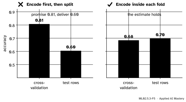
Wrong beside right. Left: the id encoded on all training rows before cross-validation; every validation fold’s encodings contain its own labels, and the estimate is \(0.81\) against \(0.60\) on test rows. Right: the encoder in a pipeline, fitted inside each fold: \(0.68\), and the test rows agree.
“Leave-one-out is enough: the row is not in its own mean.”
Its label is still in the category’s total, and the encoding is that total minus the label. As the worked example showed, a threshold reads the label off within each category.
“I target-encoded the whole training set, then cross-validated.”
Then each validation fold was encoded with its own labels, and the score is inflated, as in the figure. Put the encoder inside the pipeline that cross-validation refits on every fold.
“Ordinal codes are as good as anything for a tree.”
Only if the order means something. With an arbitrary order a tree needs several cuts to collect the categories that behave alike; a target statistic or a native categorical split puts them next to each other.
Check yourself
Recall
1. What is target leakage in a target encoding?
Show answer
A training row’s own label is used to compute its encoded feature, so the feature carries part of the answer on training rows but not on new ones.
2. For a category with \(n_c\) training rows, by how much does the greedy encoding of a training row rise, on average, when its own label is 1 instead of 0?
Show answer
By \({1/(n_c + a)}\), when the category is unrelated to the label. For a test row the difference is 0.
3. Which rows does the ordered target statistic of row \(i\) use?
Show answer
The rows of the same category that come before \(i\) in a random permutation, together with the prior.
4. How does TargetEncoder.fit_transform keep a row’s label out of its encoding?
Show answer
By cross-fitting: the training rows are split into folds, and each fold is encoded with statistics learnt on the other folds.
5. What makes a tree oblivious?
Show answer
Every node at the same depth uses the same split, so the tree is balanced, has \(2^d\) leaves at depth \(d\), and a leaf is found from \(d\) yes-or-no answers.
Exercises
1.★ With prior \(p = 0.4\) and \(a = 2\), encode a category whose training rows have labels \(1, 1, 1\), greedily. Then encode a category never seen in training.
Show solution
Greedy: \({(3 + 2 \times 0.4)/(3 + 2)} = 3.8/5 = 0.76\). An unseen category has no rows, so it gets \({(0 + 0.8)/(0 + 2)} = 0.4\), the prior.
2.★★ Encode the eight rows of the worked example in the reverse order (row 8 first). Which encodings change?
Show solution
Walking 8, 7, …, 1 with \(p = 0.5\) and \(a = 1\): row 8 (blue, 0) \(0.5\); row 7 (green, 1) \(0.5\); row 6 (red, 0) \(0.5\); row 5 (blue, 1): before it blue 0, so \(0.5/2 = 0.25\); row 4 (green, 0): before it green 1, so \(1.5/2 = 0.75\); row 3 (red, 1): before it red 0, so \(0.25\); row 2 (blue, 0): before it blue 0, 1, so \(1.5/3 = 0.5\); row 1 (red, 1): before it red 0, 1, so \(0.5\). Rows 3, 4, 6 and 7 change; rows 1, 2, 5 and 8 happen to keep their values. One order is one noisy draw, which is why CatBoost uses several permutations.
3.★★★ In a training set every category occurs exactly once, and the labels have nothing to do with the categories. Show that the greedy encodings take only two values, find a threshold that classifies every training row correctly, and find the accuracy on test rows whose categories were never seen.
Show solution
With \(n_c = 1\) the category’s label sum is the row’s own label, so \(\hat{x} = {(y + ap)/(1 + a)}\): either \({(1 + ap)/(1 + a)}\) for \(y = 1\) or \({ap/(1 + a)}\) for \(y = 0\). The first is larger by \({1/(1 + a)}\), the gap of the formal section with \(n_c = 1\). Any threshold strictly between them, for example \({(0.5 + ap)/(1 + a)}\), classifies every training row correctly. A test row of an unseen category has no training rows, so it gets \({(0 + ap)/(0 + a)} = p\), the same value for every test row. The split therefore predicts one class for all of them, and its accuracy is the share of that class among the test rows: no better than always guessing one label. This is the extreme example of Section 3.2 of the paper.
Sources. Each was opened and checked against this lesson on 15 November 2026.
Liudmila Prokhorenkova, Gleb Gusev, Aleksandr Vorobev, Anna Veronika Dorogush and Andrey Gulin, CatBoost: unbiased boosting with categorical features, NeurIPS 2018. Section 3.2 (greedy target statistics with prior \(p\) and weight \(a\), equation 4; target leakage and conditional shift; the unique-category example; property P1; holdout and leave-one-out statistics with the constant-feature example; ordered statistics along a random permutation), Section 4 (prediction shift and ordered boosting) and Section 5 (several permutations, and oblivious trees as balanced, less prone to overfitting and fast at test time).
scikit-learn developers, Ensembles, Section 1.11.1.1.4 and Preprocessing, Section 8.3.4.2, scikit-learn 1.9 User Guide. Native categorical splits with categorical_features="from_dtype", cardinality below max_bins and \(K - 1\) cuts after sorting; TargetEncoder with its shrinkage, smooth="auto" and cross-fitting in fit_transform.
LightGBM developers, Features, LightGBM documentation. Categorical splits found by sorting the categories by their accumulated statistics, with Fisher (1958) for the regression case.
CatBoost developers, Common parameters, CatBoost documentation. boosting_type (Ordered or Plain), depth and the default grow_policy SymmetricTree.
Next.ML02.5.4 The three libraries side by side maps the settings of XGBoost, LightGBM, CatBoost and scikit-learn onto one another and compares them on two datasets.