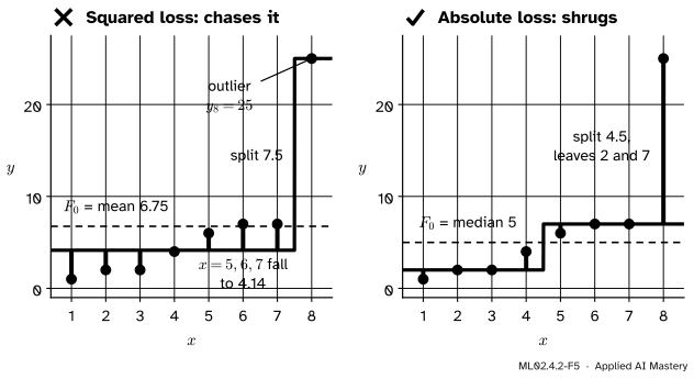
A residual is the negative gradient of the squared loss with respect to a prediction. That one fact turns boosting into gradient descent on the predictions, and lets the same loop boost the absolute and Huber losses, which shrug off an outlier that captures squared-loss boosting.
ML02.4.2L2 Intermediate25 minIn review (what this means)
The maths and code on this page are checked by automated tests on every change, but an independent reader has not signed it off yet. Spot a mistake or a confusing step? Tell us.
Show that the residual is the negative gradient of the squared loss with respect to the prediction, and compute pseudo-residuals for the absolute and Huber losses.
State the general gradient boosting algorithm and explain the role of each step: pseudo-residuals, tree fit, leaf values, update.
Derive the best leaf value for the squared loss (the mean), the absolute loss (the median) and the Huber loss (the root of a clipped sum).
Boost an eight-point set with an outlier under all three losses, from scratch and with GradientBoostingRegressor.
The question
Change one target of the eight points from \(9\) to \(25\), a typing error or a sensor glitch. Fit the first boosting stump to the residuals as before, and it spends its only split on that one point, dragging the predictions for \(x = 5, 6, 7\) down by more than two units. Can boosting be told to care less about large errors? The answer needs one change of view: a residual is a gradient.
From the last lesson
1. In least-squares boosting, what is each new stump fitted to, and what does each of its leaves hold?
Show answer
To the current residuals \({y_i - F_{m-1}(x_i)}\); each leaf holds the mean residual of its points.
2. On the eight points, which splits do the first three stages choose, and what is the training MSE after stage 3?
Show answer
\(4.5\), \(7.5\) and \(1.5\); the training MSE after stage 3 is \(0.6071\).
Intuition
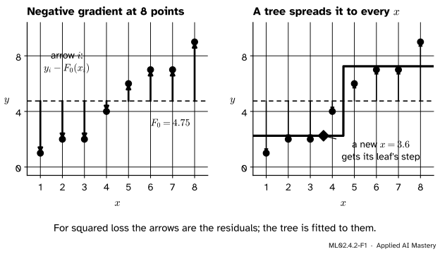
Forget trees for a moment and treat the eight predictions \(F(x_1), \dots, F(x_8)\) as eight free numbers. The loss \({\sum \tfrac12 (y_i - F(x_i))^2}\) is a function of those numbers, and gradient descent (ML01.5) would move each one downhill. The downhill direction for prediction \(i\) is exactly its residual \({y_i - F(x_i)}\).
ML02.4.2-F1
Left: the negative gradient of the loss has one component per training point, and for squared loss it is the residual. Right: a tree fitted to those components turns eight arrows into a step that is defined for every \(x\).
So the stump of the last lesson was a gradient step all along. The arrows on the left say how to move the eight training predictions. On their own they say nothing about \(x = 3.6\), which is not a training point. Fitting a tree to the arrows spreads the step to every input: the new point takes the step of the leaf it falls in. This is gradient descent in function space: the thing being moved is the function \(F\), one tree at a time.
Nothing in this ties boosting to the squared loss: any loss with a derivative gives arrows.
Build it up
Step 1. The loss as a function of the predictions. Write \(F_i\) for the prediction at the training input \(x_i\). The training loss is a sum over points, \({\sum_i L(y_i, F_i)}\), and each \(F_i\) appears in exactly one term.
Step 2. Its gradient. The partial derivative with respect to \(F_i\) is the derivative of that one term. For the squared loss \({L = \tfrac12 (y_i - F_i)^2}\) the chain rule gives \({\pd{L}{F_i} = -(y_i - F_i)}\), so the negative gradient is the residual \({y_i - F_i}\). The factor \(\tfrac12\) is there only to make this come out clean.
Step 3. A free step memorises. Gradient descent with step size \(1\) on the free numbers would set \({F_i \leftarrow F_i + (y_i - F_i) = y_i}\): every training prediction jumps to its target, and the model says nothing about any other input.
Step 4. A tree step generalises. Instead, fit a small tree to the negative gradient and step along the tree. Points in the same leaf move together, and every new input moves with its leaf.
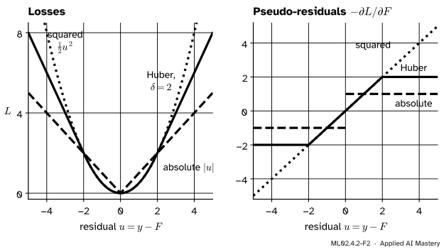
Step 5. Other losses give other arrows. Write \({u = y - F}\). The absolute loss\(\abs{u}\) has negative gradient \(\operatorname{sign}(u)\): every point pulls with the same strength, however far off it is. The Huber loss is quadratic for \({\abs{u} \le \delta}\) and linear beyond, so its negative gradient is \(u\) clipped to \({[-\delta, \delta]}\). These negative gradients are called pseudo-residuals.
ML02.4.2-F2
Three losses of the residual (left) and their negative gradients (right). Squared loss pulls in proportion to the error, absolute loss pulls with constant strength, and the Huber loss caps the pull at \(\delta\).
The formal statement
NoteAlgorithm: gradient boosting
For a differentiable loss \(L(y, F)\), training points \((x_i, y_i)\), \(M\) stages and a learning rate \(\cparam{\nu}\):
Set \(F_0\) to the constant \(c\) that minimises \({\sum_i L(y_i, c)}\).
For \(m = 1, \dots, M\):
compute the pseudo-residuals \({r_i = -\pd{L(y_i, F)}{F}}\) at \({F = F_{m-1}(x_i)}\);
fit a regression tree to the pairs \((x_i, r_i)\) by least squares; call its leaves \(R_1, \dots, R_J\);
in each leaf, choose the value \(\gamma_j\) that minimises \({\sum_{x_i \in R_j} L(y_i, F_{m-1}(x_i) + \gamma)}\);
set \({F_m(x) = F_{m-1}(x) + \cparam{\nu}\, \gamma_j}\) for every \(x\) in leaf \(R_j\).
This is Algorithm 10.3 of ESL with the learning rate of its Section 10.12.1. Step 2b uses the tree only to choose the regions; step 2c then asks the real loss what each region should predict. For the squared loss the two agree; for other losses they do not.
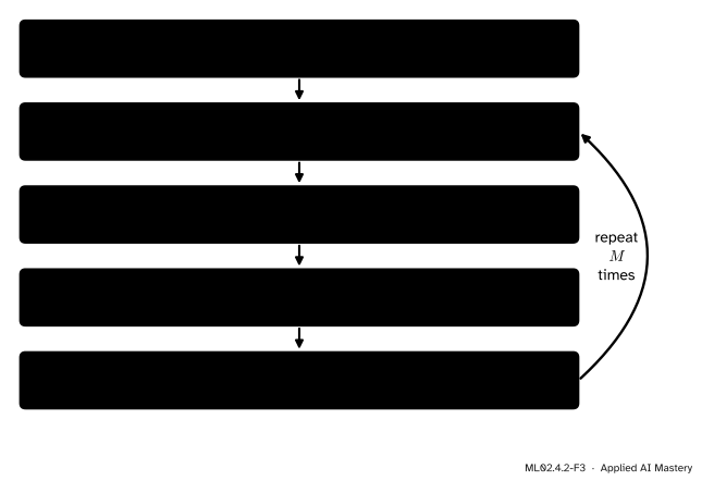
ML02.4.2-F3
The loop of gradient boosting. Only step 2a and step 2c depend on the loss.
The best leaf values. Write \(r_1, \dots, r_k\) for the ordinary residuals \({y_i - F_{m-1}(x_i)}\) of the \(k\) points in one leaf, so that step 2c minimises \({S(\gamma) = \sum L(r_i - \gamma)}\), a loss of the shifted residuals.
Squared loss.\({S(\gamma) = \sum \tfrac12 (r_i - \gamma)^2}\) has derivative \({-\sum (r_i - \gamma)}\), zero at \({\gamma = \frac1k \sum r_i}\): the mean.
Absolute loss.\({S(\gamma) = \sum \abs{r_i - \gamma}}\). Away from the \(r_i\) its slope is
because each term rises with slope \(+1\) when \(\gamma\) is above \(r_i\) and \(-1\) when it is below. The slope is negative while fewer than half the residuals lie below \(\gamma\) and positive once more than half do, so \(S\) is smallest at the median.
Huber loss. With \({\psi(u) = \min(\delta, \max(-\delta, u))}\), the clipped residual, the derivative is \({S'(\gamma) = -\sum \psi(r_i - \gamma)}\). The best \(\gamma\) solves
\[
\sum_{i=1}^{k} \psi(r_i - \gamma) = 0 .
\]
Points within \(\delta\) of \(\gamma\) count with their full residual, as in the mean; points further away count only \(\pm\delta\), as in the median. The solution lies between the two, and since \(S\) is convex a one-dimensional search finds it.
Go deeper: why the tree is fitted to the gradient and not to the loss
Step 2b could, in principle, search for the tree whose regions and values most reduce the loss itself. For the absolute or Huber loss that search has no fast algorithm. ESL (Section 10.10.2) explains the compromise: fit the tree to the negative gradient by least squares, which uses the fast split search of ML02.1.3, and accept regions that are “similar enough”. Step 2c then repairs the values.
Libraries take one more shortcut for the Huber loss. Instead of solving the clipped equation, they take one step from the median \(\tilde{r}\) of the leaf: \({\gamma \approx \tilde{r} + \frac1k \sum \psi(r_i - \tilde{r})}\). scikit-learn’s HuberLoss computes exactly this, citing Friedman (2001). It also chooses \(\delta\) afresh at every stage, as the alpha quantile of the absolute residuals (ESL Table 10.2).
Worked example
The eight points with the outlier: \(y = (1, 2, 2, 4, 6, 7, 7, 25)\). One stage of each loss, with \(\cparam{\nu} = 1\) and \(\delta = 2\) for the Huber loss.
Starting constants. The squared loss starts at the mean, \({54/8 = 6.75}\). The absolute loss starts at the median, the midpoint of \(4\) and \(6\), which is \(5\). For the Huber loss, at \(c = 5\) the clipped residuals are (−2, −2, −2, −1, 1, 2, 2, 2), which add up to \(0\), so \(5\) solves the Huber equation too.
Squared loss. The pseudo-residuals are \({y_i - 6.75}\), ending in \(18.25\) for the outlier. The split at \(7.5\) isolates it: the left seven targets have mean \({29/7 \approx 4.14}\) and squared error \({159 - 841/7 \approx 38.86}\), the right leaf has none. The split at \(4.5\) would leave the right leaf (6, 7, 7, 25) with squared error \(252.75\). So \(F_1\) is \(4.14\) up to \(x = 7\) and \(25\) at \(x = 8\): the points at \(x = 5, 6, 7\), which the mean had nearly right, are now about two units off.
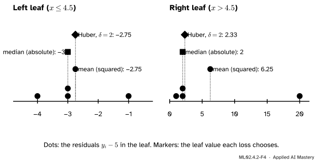
Absolute loss. The pseudo-residuals are the signs of \({y_i - 5}\): (−1, −1, −1, −1, 1, 1, 1, 1). A stump fits them perfectly at \(4.5\). Step 2c replaces its \(\pm 1\) by the median residual of each leaf: the left leaf holds (−4, −3, −3, −1), median \(-3\); the right leaf holds (1, 2, 2, 20), median \(2\). So \(F_1\) is \(2\) then \(7\).
Huber loss. The pseudo-residuals are the clipped residuals (−2, −2, −2, −1, 1, 2, 2, 2); the outlier pulls no harder than the point at \(x = 6\). The split at \(4.5\) has squared error \(1.5\), against \(6.8\) for the splits at \(3.5\) and \(5.5\). In the left leaf, \({\gamma = -2.75}\) leaves every residual within \(\delta\), and the deviations (−1.25, −0.25, −0.25, 1.75) add up to \(0\). In the right leaf, guess that only the outlier is clipped:
The guess holds: \({1 - 7/3}\) and \({2 - 7/3}\) are within \(2\) of zero, and \({20 - 7/3}\) is not. So \(F_1\) is \({5 - 2.75 = 2.25}\) then \({5 + 7/3 \approx 7.33}\).
ML02.4.2-F4
Where each loss puts the leaf. In the right leaf the outlier at \(20\) drags the mean to \(6.25\); the median ignores it and the Huber value moves only a third of a unit.
Code
One function covers all three losses: each loss supplies its starting constant, its pseudo-residuals and its leaf value.
import numpy as npfrom scipy.optimize import brentqx = np.arange(1.0, 9.0)y = np.array([1, 2, 2, 4, 6, 7, 7, 25], dtype=float) # the last target is an outlierDELTA =2.0def huber_value(r, delta=DELTA):"""The gamma that solves sum(clip(r - gamma, -delta, delta)) = 0."""return brentq(lambda g: np.clip(r - g, -delta, delta).sum(), r.min() -1, r.max() +1)LOSSES = {"squared": (np.mean, lambda u: u, np.mean),"absolute": (np.median, np.sign, np.median),"huber": (huber_value, lambda u: np.clip(u, -DELTA, DELTA), huber_value),}def best_split(x, r): values = np.unique(x) cuts = (values[:-1] + values[1:]) /2 sse = [((r[x <= s] - r[x <= s].mean()) **2).sum() + ((r[x > s] - r[x > s].mean()) **2).sum() for s in cuts]return cuts[int(np.argmin(sse))]def gradient_boost(x, y, loss, stages, nu=1.0): start, pseudo, leaf_value = LOSSES[loss] pred = np.full(len(y), start(y))for _ inrange(stages): s = best_split(x, pseudo(y - pred)) # 2a and 2b: tree fitted to the gradient u = y - pred left = x <= s pred = pred + nu * np.where(left, leaf_value(u[left]), leaf_value(u[~left])) # 2c and 2dreturn predfor loss in LOSSES:print(f"{loss:9s}", np.round(gradient_boost(x, y, loss, stages=1), 3))
Now scikit-learn. With loss="absolute_error" it starts from the median and sets each leaf to the median residual. With loss="huber", \(\delta\) is the alpha quantile of the absolute residuals \({\abs{y_i - 5}}\), sorted 1, 1, 2, 2, 3, 3, 4, 20. The library takes the smallest value with at least that fraction of the list at or below it, so alpha=0.5 gives the fourth value, \(2\).
from sklearn.ensemble import GradientBoostingRegressorX = x.reshape(-1, 1)for loss, extra in [("squared_error", {}), ("absolute_error", {}), ("huber", {"alpha": 0.5})]: gbr = GradientBoostingRegressor(loss=loss, n_estimators=1, learning_rate=1.0, max_depth=1, **extra)print(f"{loss:15s}", np.round(gbr.fit(X, y).predict(X), 3))
The squared and absolute rows match the scratch code. The Huber row gives \(7.25\) in the right leaf, not \(7.33\): the one-step shortcut of the .deeper block, the median \(2\) plus the mean clipped deviation \(0.25\). With the default alpha=0.9, \(\delta\) is the eighth value, \(20\): nothing is clipped, and the first split lands on the outlier again.
Explore
The module’s interactive, the residual stepper, lives in lesson ML02.4.1. Its bars are the squared-loss pseudo-residuals: the arrows of this lesson’s anchor figure.
Pitfalls
ML02.4.2-F5
Wrong beside right, after one stage. The squared loss spends its first split on the outlier and makes three good predictions worse; the absolute loss splits where the data change and leaves the outlier alone.
“Gradient boosting does gradient descent on the trees’ parameters.”
No parameter is differentiated. The gradient is taken with respect to the predictions\(F(x_1), \dots, F(x_n)\), one number per training point. The tree is then fitted to that gradient by an ordinary split search, which has no gradient at all.
“The tree fitted to the pseudo-residuals is the update.”
Only its regions are. For the absolute loss the tree is fitted to signs and its leaves hold numbers between \(-1\) and \(1\), which would move every prediction by at most one unit. Step 2c replaces them with the median residual of each leaf, \(-3\) and \(2\) in the worked example.
“A robust loss is always the better choice.”
With clean, roughly Gaussian errors a mean is more accurate than a median, so squared loss wins. The Huber loss is the compromise, and its \(\delta\) decides which it resembles; scikit-learn’s default alpha=0.9 still let the outlier take the first split here.
Check yourself
Recall
1. What is the negative gradient of \({\tfrac12 (y_i - F_i)^2}\) with respect to \(F_i\)?
Show answer
\({y_i - F_i}\), the residual. The derivative is \({-(y_i - F_i)}\) by the chain rule, and the minus sign cancels.
2. What are the pseudo-residuals of the absolute loss and of the Huber loss?
Show answer
For the absolute loss, \({\operatorname{sign}(y_i - F_i)}\). For the Huber loss, \({y_i - F_i}\) clipped to the interval \({[-\delta, \delta]}\).
3. Why fit a tree to the negative gradient instead of stepping each training prediction by it?
Show answer
A free step only moves the training predictions, and with step size \(1\) it memorises the targets. A tree turns the step into a function of \(x\), so new inputs move too.
4. Which leaf value minimises the absolute loss over a leaf, and why?
Show answer
The median of the leaf’s residuals. The slope of \({\sum \abs{r_i - \gamma}}\) is the number of residuals below \(\gamma\) minus the number above, which changes sign at the median.
5. In the worked example, what do the squared, absolute and Huber losses predict for \(x = 6\) after one stage?
Show answer
About \(4.14\) (squared), \(7\) (absolute) and about \(7.33\) (Huber, \(\delta = 2\)). The target is \(7\).
Exercises
1.★ A leaf holds the residuals (−1, 0, 3, 10). Find its value under the squared loss, the absolute loss and the Huber loss with \(\delta = 2\).
Show solution
Squared: the mean, \({12/4 = 3}\). Absolute: the median, the midpoint of \(0\) and \(3\), which is \(1.5\). Huber: guessing that only \(10\) is clipped gives \({\gamma = 4/3}\), but then \({-1 - 4/3}\) is beyond \(-2\), so \(-1\) is clipped too. Then \({-2 + (0 - \gamma) + (3 - \gamma) + 2 = 0}\), so \({\gamma = 1.5}\). Check: the deviations \(-2.5\), \(-1.5\), \(1.5\), \(8.5\) are clipped exactly at the ends. The Huber value is \(1.5\).
2.★★ The quantile loss with level \(\tau\) charges \({\tau u}\) when \({u = y - F \ge 0}\) and \({(\tau - 1) u}\) when \({u < 0}\). Find its pseudo-residuals and show that the best constant in a leaf is a \(\tau\) quantile of the residuals.
Show solution
For \(u > 0\) the loss is \({\tau (y - F)}\), with derivative \({-\tau}\) in \(F\); for \(u < 0\) it is \({(\tau - 1)(y - F)}\), with derivative \({1 - \tau}\). So the pseudo-residual is \(\tau\) when the prediction is too low and \({\tau - 1}\) when it is too high. For a constant \(\gamma\), the slope of \({\sum \rho_\tau(r_i - \gamma)}\) is \({(1 - \tau)\,\#\{r_i < \gamma\} - \tau\,\#\{r_i > \gamma\}}\). With \(k\) residuals and a fraction \(q\) of them below \(\gamma\), this is \({k\,[(1 - \tau) q - \tau(1 - q)]}\), which is \({k\,(q - \tau)}\). It changes sign where \({q = \tau}\), at a \(\tau\) quantile. For \({\tau = \tfrac12}\) this is the median and the absolute loss, halved.
3.★★★ Run a second stage of absolute-loss boosting on the outlier set, starting from \({F_1 = (2, 2, 2, 2, 7, 7, 7, 7)}\). Give the pseudo-residuals, a best split, the leaf medians and \(F_2\). Is the split unique?
Show solution
The residuals \({y - F_1}\) are (−1, 0, 0, 2, −1, 0, 0, 18), so the pseudo-residuals are their signs, (−1, 0, 0, 1, −1, 0, 0, 1). The total of their squares is \(4\) and their sum is \(0\). A split with left sum \(a\) over \(k\) points has squared error \({4 - a^2/k - a^2/(8 - k)}\), since the right sum is \(-a\). The cumulative sums from the left are −1, −1, −1, 0, −1, −1, −1 for \(k = 1, \dots, 7\), so \(a^2 = 1\) except at \(k = 4\), and \({1/k + 1/(8 - k)}\) is largest at \(k = 1\) and \(k = 7\), where it is \(8/7\). Splits at \(1.5\) and \(7.5\) tie, with squared error \({4 - 8/7 = 20/7}\): the split is not unique. At \(1.5\) the leaves hold the residuals \((-1)\) and (0, 0, 2, −1, 0, 0, 18), with medians \(-1\) and \(0\), so \({F_2 = (1, 2, 2, 2, 7, 7, 7, 7)}\). At \(7.5\) the medians are \(0\) and \(18\), which gives \({F_2 = (2, 2, 2, 2, 7, 7, 7, 25)}\), chasing the outlier after all. The first split found in a left to right search is \(1.5\), so the scratch code above returns the first answer.
Summary card
Boosting is gradient descent on the predictions, with a tree to carry each step to new inputs.
ML02.4.2-F1
Arrows at the points, then a tree.
Pseudo-residuals.\({r_i = -\pd{L(y_i, F)}{F}}\) at \({F = F_{m-1}(x_i)}\).
Loop. Tree on the \(r_i\) for the regions, the loss for the leaf values, then add \({\cparam{\nu}\,\gamma_j}\).
Sources and next steps
Sources. Each was opened and checked against this lesson on 15 November 2026.
Trevor Hastie, Robert Tibshirani and Jerome Friedman, The Elements of Statistical Learning, 2nd edition, 12th printing. Section 10.10 treats the fitted values at the \(N\) training points as the parameters of a numerical optimisation, with the gradient components (10.35), and fits a tree to the negative gradient by least squares (10.37). Table 10.2 lists the negative gradients of the squared, absolute and Huber losses, with \(\delta\) an \(\alpha\) quantile of the absolute residuals, and Algorithm 10.3 (page 361) is the loop of this lesson. Section 10.9 notes that for absolute loss the leaf value is the median of the residuals. ESL’s Huber loss (10.23) is twice the one used here, which changes neither its minimiser nor its regions.
Kilian Weinberger, Lecture 19: Boosting, Cornell CS4780, Fall 2018. Describes boosting as gradient descent in function space, with the residual as the target for squared loss.
scikit-learn developers, User Guide 1.11.1.2.3, version 1.9.1. Each tree is fitted to the negative gradients, “some kind of gradient descent in a functional space”, and for 'absolute_error' the leaves are then reset to the median. The one-step Huber leaf value was read in the library’s own source, HuberLoss.fit_intercept_only in sklearn/_loss/loss.py.