Bagging grows a deep tree on each bootstrap sample of one data set and lets the trees vote or average. Derive why a bootstrap sample holds about 63.2 % of the points, bag trees by hand and in NumPy, and see why it helps trees but not a straight line.
ML02.2.2L2 Intermediate25 minIn review (what this means)
The maths and code on this page are checked by automated tests on every change, but an independent reader has not signed it off yet. Spot a mistake or a confusing step? Tell us.
Draw a bootstrap sample and derive that it holds on average a fraction 1 − (1 − 1/n)ⁿ of the distinct points, which tends to 1 − 1/e.
Bag deep trees by hand on a small regression set and from scratch in NumPy on the twelve points.
Explain with the variance formula why bagging helps unstable learners such as deep trees and barely changes stable ones such as linear regression.
Fit a BaggingClassifier and read its vote shares.
The question
The averaging of the last lesson needs many predictors trained on different data sets. In practice there is only one data set. How can one data set produce many different trees, and does averaging them still help?
From the last lesson
1. What is the variance of the average of \(B\) predictors with variance \(\sigma^2\) and pairwise correlation \(\rho\)?
Show answer
\(\rho\sigma^2 + {(1-\rho)\sigma^2/B}\).
2. What two things does an ensemble need from its members?
Show answer
Each member must be good on its own, and the members must disagree, so that their errors are not all shared.
Intuition
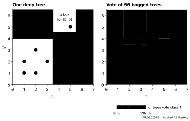
Draw a new data set from the one you have: pick \(n\) points at random with replacement. Some points come up twice, some not at all. Grow a deep tree on it, and repeat. Each tree has seen a slightly different data set, so each makes slightly different mistakes, and the vote cancels many of them.
ML02.2.2-F1
The twelve points. One deep tree gives every odd point a box of its own. Fifty trees, each grown on a bootstrap sample, vote: where they agree the shading is white or dark, and around the two odd points the vote is split.
This is bagging, short for bootstrap aggregating: bootstrap samples to make the members, aggregation (a vote or an average) to combine them.
Build it up
Step 1. A bootstrap sample. Number the points 1 to \(n\). Draw \(n\) times, each time picking every number with chance \(1/n\), and put the drawn point in the sample. Lesson S02.8 used the same resampling to measure how much a statistic varies; here it makes the members of an ensemble.
ML02.2.2-F2
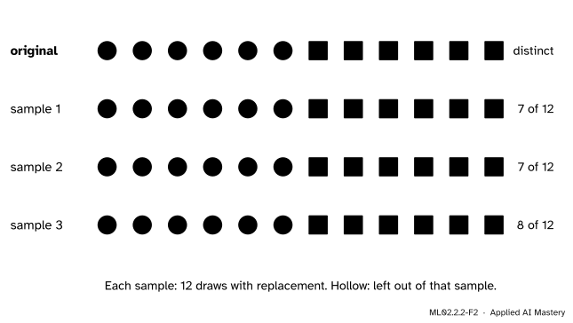
The first three bootstrap samples of the twelve points used in this lesson. Each has twelve draws; the repeats push other points out, so each holds only 7 or 8 distinct points.
Step 2. Grow a deep tree on each sample. Grow it as in ML02.1.3, until every leaf is pure. A repeated point simply counts more in the impurity of its node.
Step 3. Aggregate. For regression, average the \(B\) trees’ predictions. For classification, let each tree vote and take the majority; the share of votes for a class is a rough probability.
Step 4. Why it should help. The bootstrap samples are like fresh data sets, so each tree is a noisy predictor with some variance \(\sigma^2\), and by the last lesson their average has less. They are not truly fresh, though: any two samples share most of their points, so the trees are correlated and the variance stops at \(\rho\sigma^2\). Bagging buys the \(1/B\) part, not more.
The formal statement
NoteDefinition: bagging
Given training data of \(n\) examples, draw \(B\) bootstrap samples, each of \(n\) examples drawn with replacement, and fit a model \(\hat{f}^{*m}\) to sample \(m\). The bagged regression prediction is
and the bagged classifier predicts the class that most of the \(B\) classifiers vote for.
How much of the data is in one sample? Fix one point, \(i\). On a single draw it is missed with chance \(1 - 1/n\). The \(n\) draws are independent, so it is missed by all of them with chance
\[
\Prob(i \text{ left out}) = \Big(1 - \frac{1}{n}\Big)^{n}.
\]
Let \(I_i\) be 1 if point \(i\) is in the sample and 0 if not. The number of distinct points in the sample is \(I_1 + \dots + I_n\), and the expected value of a sum is the sum of the expected values, whether or not the \(I_i\) are independent. Each \(I_i\) has expected value \(1 - {(1 - 1/n)^n}\), so
For the twelve points, \({(11/12)^{12}} = 0.352\), so a sample holds on average \({12 \times 0.648} = 7.78\) distinct points; the three samples above held 7, 7 and 8.
The limit. Take logarithms: \({\ln\big((1 - 1/n)^n\big)} = {n\ln(1 - 1/n)}\). Put \(u = 1/n\), which goes to 0 as \(n\) grows:
As \(u \to 0\) this is the slope of \({\ln(1 - u)}\) at \(u = 0\), which is \({-1/(1 - 0)} = -1\). So \({(1 - 1/n)^n} \to e^{-1} \approx 0.368\), and a large bootstrap sample holds about \(1 - e^{-1} \approx 0.632\) of the distinct points.
ML02.2.2-F3
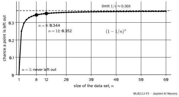
The chance \({(1 - 1/n)^n}\) that a given point is missing from a bootstrap sample. Already at \(n = 8\) it is 0.344; it creeps up to \(1/e\).
When bagging helps. The bagged prediction is an average, so by the last lesson its variance is \(\rho\sigma^2 + {(1 - \rho)\sigma^2/B}\), while its mean stays close to that of one tree on a bootstrap sample. The gain is the part \({(1-\rho)\sigma^2(1 - 1/B)}\) that averaging removes, and it is large only when \(\sigma^2\) is large and \(\rho\) is not close to 1. A deep tree is unstable: removing or repeating a few points moves its splits and changes its predictions a lot, so \(\sigma^2\) is large and the trees on different samples differ. Their average is a new, smoother model that no single tree could be.
A stable method gains nothing. Take the simplest, the sample mean. On average over bootstrap samples every point is drawn once, so the bootstrap means average out, as \(B\) grows, to exactly the original mean: bagging gives back what you had. Each bootstrap mean is noisier than the original, and any two are only about 50 % correlated, but the noise they add is exactly what averaging removes again. A least-squares line behaves almost the same way, as the code below shows.
Worked example
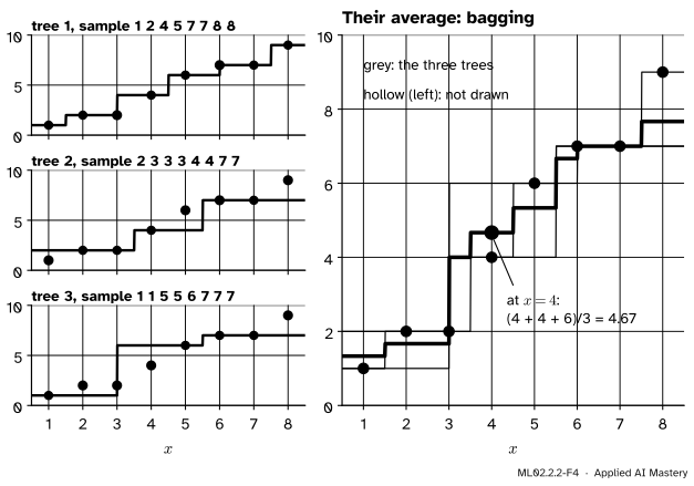
Bag three deep regression trees on the eight-point set by hand. The data are \(x = 1, \dots, 8\) and \(y = {(1, 2, 2, 4, 6, 7, 7, 9)}\). The code below draws three bootstrap samples:
A deep tree on one feature splits halfway between neighbouring sampled values until each leaf is pure, so it predicts the \(y\) of the nearest sampled \(x\). A point exactly halfway between two sampled values goes left, because a split sends \(x \leq\) threshold left. For tree 1 at \(x = 3\): the nearest sampled values are 2 and 4, the split is at 3, and 3 goes left to \(y = 2\). For tree 2 at \(x = 5\) there is no tie: the nearest sampled values are 4 and 7, the split is at 5.5, and 5 is nearer to 4, so it gets \(y = 4\).
\(x\)
T1
T2
T3
mean
1
1
2
1
1.33
2
2
2
1
1.67
3
2
2
1
1.67
4
4
4
6
4.67
5
6
4
6
5.33
6
6
7
7
6.67
7
7
7
7
7
8
9
7
7
7.67
At \(x = 4\) the trees say 4, 4 and 6, so the bagged prediction is \(14/3 \approx 4.67\). Tree 3 never saw \(x = 4\) and copied its neighbour at 5; the other two outvote it only partly.
ML02.2.2-F4
The worked example. Each tree is a staircase through the points it drew. The average is a finer staircase with smaller steps: no single tree’s jump survives whole.
The bagged staircase has smaller steps than any one tree. With 200 trees from the same random stream the steps are finer still, and the prediction at \(x = 4\) becomes 3.59.
Code
From scratch: the grower of ML02.1.3 in a compact form, bootstrap samples, and a vote.
import numpy as npX = np.array([(1, 1), (2, 1), (1, 2), (2, 3), (3, 2), (5, 5), (4, 1), (5, 2), (5, 3), (4, 4), (2, 5), (6, 5)], dtype=float)y = np.array([0] *6+ [1] *6)def gini(labels): p = np.bincount(labels, minlength=2) /len(labels)return1- np.sum(p **2)def grow(X, y):"""A fully grown tree: best Gini split at every node, first one found wins a tie, stop when pure."""if gini(y) ==0:return {"leaf": int(y[0])} best =Nonefor j inrange(X.shape[1]): values = np.unique(X[:, j])for s in (values[:-1] + values[1:]) /2: left = X[:, j] <= s score = (left.sum() * gini(y[left]) + (~left).sum() * gini(y[~left])) /len(y)if best isNoneor score < best[0] -1e-12: best = (score, j, s) _, j, s = best left = X[:, j] <= sreturn {"j": j, "s": s, "left": grow(X[left], y[left]), "right": grow(X[~left], y[~left])}def predict(tree, x):while"leaf"notin tree: tree = tree["left"] if x[tree["j"]] <= tree["s"] else tree["right"]return tree["leaf"]rng = np.random.default_rng(0)samples = [rng.integers(0, 12, size=12) for _ inrange(50)]trees = [grow(X[idx], y[idx]) for idx in samples]share = np.array([[predict(t, x) for t in trees] for x in X]).mean(axis=1) # share voting class 1print("distinct points per sample, on average:", np.mean([len(set(s)) for s in samples]))print("share of trees voting 1 at each point:", share.round(2))print("training errors of the vote:", int(np.sum((share >0.5) != y)))
distinct points per sample, on average: 7.92
share of trees voting 1 at each point: [0.   0.06 0.02 0.16 0.04 0.44 0.82 0.9  0.9  0.92 0.68 0.88]
training errors of the vote: 0
The odd circle at (5, 5) gets 44 % of the votes for class 1: most trees that drew it put it in a box of its own, the others did not. Now the regression trees of the worked example.
xs = np.arange(1, 9, dtype=float)ys = np.array([1, 2, 2, 4, 6, 7, 7, 9], dtype=float)def grow_reg(x, y):"""A deep regression tree on one feature: squared-error splits until a node cannot be split."""if np.all(y == y[0]) or np.all(x == x[0]):return {"leaf": y.mean()} values = np.unique(x) sse =lambda part: ((part - part.mean()) **2).sum() s =min((values[:-1] + values[1:]) /2, key=lambda s: sse(y[x <= s]) + sse(y[x > s]))return {"s": s, "left": grow_reg(x[x <= s], y[x <= s]), "right": grow_reg(x[x > s], y[x > s])}def predict_reg(tree, x):while"leaf"notin tree: tree = tree["left"] if x <= tree["s"] else tree["right"]return tree["leaf"]rng = np.random.default_rng(1)draws = [rng.integers(0, 8, size=8) for _ inrange(200)]P = np.array([[predict_reg(grow_reg(xs[d], ys[d]), x) for x in xs] for d in draws])print("three trees:\n", P[:3])print("bagged, B = 3: ", P[:3].mean(axis=0).round(2))print("bagged, B = 200:", P.mean(axis=0).round(3))
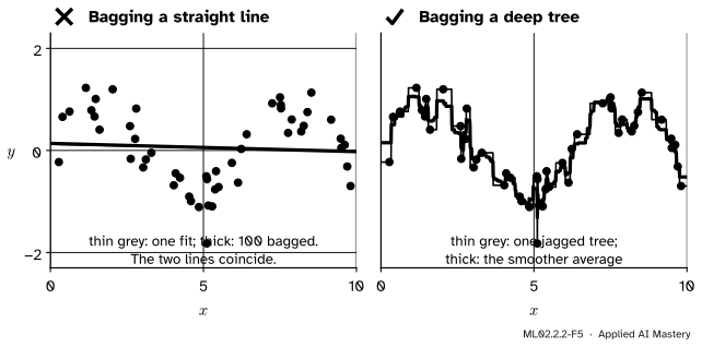
The library version is BaggingClassifier; its default member is a fully grown DecisionTreeClassifier. Then the stable-against-unstable test: a straight line and a deep tree, each alone and bagged, on 50 noisy points from a sine curve, scored on 2,000 fresh points.
library vote share for class 1 at (5, 5): 0.42   training accuracy: 1.0
line          test MSE 0.605
bagged lines  test MSE 0.604
tree          test MSE 0.264
bagged trees  test MSE 0.210
Bagging leaves the line’s test error where it was (0.605 and 0.604) and cuts the tree’s from 0.264 to 0.210. The noise alone contributes \(0.4^2 = 0.16\), so the part of the tree’s error that a model could remove fell from about 0.10 to about 0.05.
Explore
ML02.2-X1
Vote grid
Add trees one at a time with the step button and watch the shading settle and the training error fall to zero or close to it while the out-of-bag error stays well above it. Show one tree to see its bootstrap sample (hollow points were left out), then switch to the forty noisy points and turn feature subsampling on.
Pitfalls
ML02.2.2-F5
Wrong beside right. Bagging a stable method gives back the same model. Bagging an unstable one gives a smoother model with lower test error.
“Bagging improves any model.”
Only a model whose fit changes a lot when the data change a little. The bagged lines above match the single line to the third decimal in test error. Breiman’s original report found that bagging helps unstable procedures and can even slightly degrade stable ones.
“A bootstrap sample of \(n\) points has \(n\) different points.”
It has \(n\)draws, about 63 % of them distinct for large \(n\). The rest are repeats. The missing 37 % are not wasted: the last lesson of this module uses them to measure error.
“The bagged model is a tree, so I can read it like one.”
It is an average of trees, and no single tree in it gives its predictions. The cost of bagging is that the simple, readable structure of one tree is lost.
Check yourself
Recall
1. What is a bootstrap sample of a data set of \(n\) points?
Show answer
\(n\) points drawn at random with replacement from the data set, so some appear more than once and some not at all.
2. What fraction of the distinct points does a large bootstrap sample hold on average?
Show answer
\(1 - {(1 - 1/n)^n}\), which tends to \(1 - 1/e \approx 0.632\).
3. How does bagging combine its trees for regression and for classification?
Show answer
It averages their predictions for regression and takes a majority vote for classification.
4. Why does bagging help a deep tree much more than a linear regression?
Show answer
A deep tree is unstable, so trees on different samples differ and their average is a smoother model with less variance. The average of least-squares lines over bootstrap samples lands almost exactly on the original line, so bagging gives back the model you had.
5. In the worked example, what do the three trees predict at \(x = 4\), and what is the bagged prediction?
Show answer
4, 4 and 6, so the bagged prediction is \(14/3 \approx 4.67\).
Exercises
1.★ For a data set of 8 points, what is the chance that a given point is left out of a bootstrap sample, and how many distinct points does a sample hold on average?
Show solution
\({(7/8)^8} = 0.344\), so a point is in the sample with chance \(0.656\) and a sample holds on average \({8 \times 0.656} = 5.25\) distinct points. The three samples of the worked example held 6, 4 and 4.
2.★★ In the worked example, compute the bagged prediction at \(x = 1\) and at \(x = 8\), and explain why tree 2 predicts 2 at \(x = 1\).
Show solution
At \(x = 1\) the trees say 1, 2 and 1, so the average is \(4/3 \approx 1.33\). At \(x = 8\) they say 9, 7 and 7, so the average is \(23/3 \approx 7.67\). Sample 2 has no point at \(x = 1\); its smallest value is \(x = 2\) with \(y = 2\), so every input to the left of the first split falls in that leaf.
3.★★★ Show that the number of points left out of a bootstrap sample of size \(n\) has expected value \({n(1 - 1/n)^n}\), and find its value for \(n = 12\). Are the events “point 1 left out” and “point 2 left out” independent?
Show solution
Let \(J_i\) be 1 if point \(i\) is left out. Its expected value is \({(1 - 1/n)^n}\), and the number left out is \(J_1 + \dots + J_n\), so its expected value is \({n(1 - 1/n)^n}\) by linearity. For \(n = 12\) this is \({12 \times 0.352} = 4.22\). The events are not independent: both are left out when every draw misses both, which has chance \({(1 - 2/n)^n}\), and
because \({(1 - 1/n)^2} = 1 - 2/n + 1/n^2\) is larger than \(1 - 2/n\). Knowing that point 1 is out makes it a little less likely that point 2 is out too, since its draws had to land somewhere.
Summary card
Bagging: grow a deep tree on each bootstrap sample, then vote or average.
ML02.2.2-F1
One tree’s boxes, and the vote of fifty.
Bootstrap sample.\(n\) draws with replacement; a point is left out with chance \({(1 - 1/n)^n} \to 1/e \approx 0.368\).
Bagged prediction.\({\hat{f}_{\text{bag}}(\vect{x})} = {\frac{1}{B}\sum_m \hat{f}^{*m}(\vect{x})}\), or a majority vote.
When it helps. Unstable learners (deep trees), where \(\sigma^2\) is large and the members differ.
Sources. Each was opened and checked against this lesson on 15 November 2026.
Trevor Hastie, Robert Tibshirani and Jerome Friedman, The Elements of Statistical Learning, 2nd edition, corrected 12th printing. Section 8.7 defines bagging as the average of the bootstrap predictions, equation (8.51), and says that bagging can dramatically reduce the variance of unstable procedures like trees; Section 7.11, equation (7.55), gives the chance \(1 - {(1 - 1/N)^N} \approx 0.632\) that an observation is in a bootstrap sample; Section 15.2 notes that bagging does not change linear estimates such as the sample mean, and that the pairwise correlation between bootstrapped means is about 50 % (Exercise 15.4).
Leo Breiman, Bagging Predictors, Technical Report 421, Department of Statistics, University of California, Berkeley, 1994 (published in Machine Learning 24, 123 to 140, 1996). Section 1: improvement occurs for unstable procedures, where a small change in the data makes a large change in the predictor, and bagging can slightly degrade stable procedures.
scikit-learn developers, User Guide, Section 1.11.3: Bagging meta-estimator. Bagging reduces the variance of a base estimator and works best with strong, complex models such as fully developed decision trees; BaggingClassifier and BaggingRegressor.