Score every candidate on the same repeated stratified folds, compare them fold by fold, and correct the standard error for the overlap between folds. A difference smaller than that error decides nothing, and the best of many tuned models is always flattered.
ML02.11.3L2 Intermediate25 minIn review (what this means)
The maths and code on this page are checked by automated tests on every change, but an independent reader has not signed it off yet. Spot a mistake or a confusing step? Tell us.
Compare several pipelines on the same repeated stratified folds, with every preprocessing step inside the pipeline.
Derive why the naive standard error of a mean of fold differences is too small, and compute Nadeau and Bengio’s corrected one.
Decide whether a difference between two models is real, using the rule of two corrected standard errors.
Explain why the best cross-validated score among many tuned models overstates that model, and name nested cross-validation as the remedy.
The question
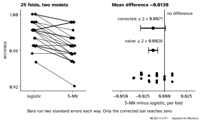
On the 569 breast-cancer patients, logistic regression scores \(0.979\) and 5-nearest neighbours \(0.966\), averaged over 25 folds. \(k\)-NN loses on 19 of the 25 folds and wins on only 3. Surely that settles it? The answer is no, and the reason is that the 25 folds are not 25 independent experiments.
From the last lesson
1. Why does standardising not change a decision tree?
Show answer
A split asks whether \(x_j \le s\), and a strictly increasing change of units keeps that answer for every row; standardising also keeps the midpoints, so the same tree results.
2. Which tables did the Grinsztajn, Oyallon and Varoquaux benchmark leave out?
Show answer
Among others: tables a default linear model already fits nearly as well as the best, rows with missing values, categories with over 20 levels, and tables under 3,000 rows.
Intuition
ML01.10.3 compared models on the same five folds and looked at the differences fold by fold, because a hard fold is hard for every model. Repeating the five folds with fresh shuffles gives more differences. It does not give that many more independent ones, because every repeat reuses the same patients.
ML02.11.3-F1
Two models on the same 25 folds. The naive error bar treats the 25 differences as independent and calls the gap decided. Corrected for the overlap between folds, the bar reaches zero.
The difference itself, \(-0.013\), is about one and a half patients in a fold of 114. The question is whether that would survive a fresh set of patients.
Build it up
Step 1. Every model on the same folds. A comparison is fair only if every candidate is trained and scored on exactly the same rows. Fix the folds once, then loop over the models.
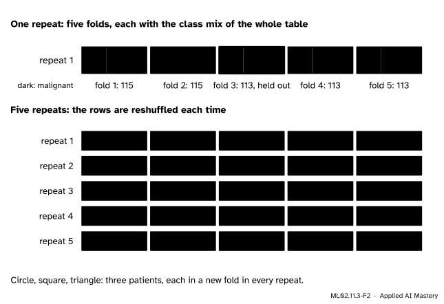
Step 2. Stratify. With 212 malignant and 357 benign patients, a fold drawn at random could hold a few too many of either. Stratified folds deal each class round the folds separately, so every fold keeps the mix of the whole table.
ML02.11.3-F2
Repeated stratified five-fold cross-validation. Each fold keeps the class mix, and each repeat reshuffles who is held out together.
Step 3. Repeat. One set of five folds depends on one shuffle. Repeat the whole thing \(r\) times with new shuffles and you have \(J = 5r\) scores per model: here \(r = 5\) and \(J = 25\).
Step 4. Everything inside the pipeline. Scaling, imputing and choosing features are part of the model. Each is fitted on the training folds of each split, inside a Pipeline, never once on all the rows (ML01.10.2).
Step 5. Compare fold by fold. For models A and B, take the 25 differences \(d_j = {b_j - a_j}\). Their mean is the gap (ML01.10.3), and their spread says how sure we are of it. But the 25 values are correlated: two training sets of the same repeat share three of their four folds, and every repeat uses the same 569 patients. The naive standard error, sd\(/\sqrt{25}\), pretends otherwise.
Step 6. Tuning flatters the winner. Try 30 settings and report the best score, and you report the one that was luckiest on these folds. The formal section measures the overlap; the pitfalls measure the luck.
The formal statement
NoteSetting
Two models are scored on the same \(J = rk\) splits (\(r\) repeats of \(k\) folds), giving differences \(d_1, \dots, d_J\). Their mean is \(\bar{d}\) and their sample standard deviation is \(s\). Suppose each \(d_j\) has variance \(\sigma^2\) and any two have correlation \(\rho\).
Result 1: the variance of the mean. The variance of a sum is the sum of all variances and covariances: \(J\) variances \(\sigma^2\), and \({J(J - 1)}\) covariances \(\rho\sigma^2\). So
This is the formula of ML02.2.1 for the average of correlated trees. More repeats shrink the second term, never the first.
Result 2: the sample variance sees only part of it. Take the mean of the \(d_j\) to be zero, which does not change any spread. Then \(\E[d_j^2] = \sigma^2\), and \(\E[\bar{d}^2]\) is \(\text{Var}(\bar{d})\) from Result 1. Since \(s^2\) is \({\sum_j (d_j - \bar{d})^2} = {\sum_j d_j^2 - J\bar{d}^2}\) divided by \(J - 1\), taking expectations gives
The naive standard error \(s/\sqrt{J}\) keeps only the \(1/J\). Nadeau and Bengio could not measure \(\rho\), so they argued for a simple stand-in, the test share \(\rho \approx n_\text{test}/n\), which makes \({\rho/(1 - \rho)} = {n_\text{test}/n_\text{train}}\). With \(k\) folds that is \({1/(k - 1)}\):
For \(J = 25\) and \(k = 5\) the factor is \(\sqrt{0.04 + 0.25} = 0.539\), against \(0.2\) for the naive \(1/\sqrt{25}\): the corrected error is 2.7 times larger.
Decision rule. Call a difference decided when \({\abs{\bar{d}}} > {2\,\text{SE}_\text{corr}}\). Otherwise the data have not separated the two models, and something else (simplicity, cost, the checklist of Lesson 2) must choose.
ML02.11.3-F5
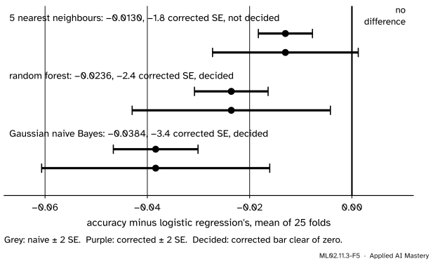
Every model against logistic regression. With naive bars all three gaps look certain. Corrected, the forest and naive Bayes are still behind, and \(k\)-NN is undecided.
Go deeper: how good is the stand-in for the correlation?
Nadeau and Bengio derived the correction for \(J\) independent random train–test splits, and noted that it can err either way, depending on whether the true \(\rho\) is above or below \(n_\text{test}/n\). In their simulations its tests were far better calibrated than the naive \(t\)-test, which rejects far too often. scikit-learn’s worked example applies the same factor to repeated \(k\)-fold, as here. Treat two corrected standard errors as a sober rule of thumb, not an exact 95 percent test.
Worked example
Six differences by hand. Two models on two repeats of three folds give the differences, in percentage points of accuracy, B minus A: \(3, 1, -1, 4, 2, 3\).
ML02.11.3-F3
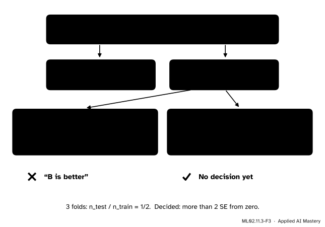
One set of differences, two standard errors. The naive one declares a winner; the corrected one does not.
and the mean is \(2.0/1.46 = 1.4\) standard errors from zero. Not decided. B may be better, but these six folds cannot show it.
Code
From scratch: stratified folds, repeated, and one loop that scores four models on the same splits.
import numpy as npfrom sklearn.datasets import load_breast_cancerfrom sklearn.ensemble import RandomForestClassifierfrom sklearn.linear_model import LogisticRegressionfrom sklearn.naive_bayes import GaussianNBfrom sklearn.neighbors import KNeighborsClassifierfrom sklearn.pipeline import make_pipelinefrom sklearn.preprocessing import StandardScalerX, y = load_breast_cancer(return_X_y=True)def stratified_folds(y, k, repeats, seed):"""Each class shuffled and dealt round the k folds; the whole thing repeated.""" rng = np.random.default_rng(seed) splits = []for _ inrange(repeats): fold_of = np.empty(len(y), dtype=int)for label in np.unique(y): members = rng.permutation(np.flatnonzero(y == label)) fold_of[members] = np.arange(len(members)) % k splits += [(np.flatnonzero(fold_of != f), np.flatnonzero(fold_of == f)) for f inrange(k)]return splitsmodels = {"logistic": lambda: make_pipeline(StandardScaler(), LogisticRegression()), # scaling inside"5-NN": lambda: make_pipeline(StandardScaler(), KNeighborsClassifier()),"naive Bayes": lambda: GaussianNB(),"forest": lambda: RandomForestClassifier(n_estimators=100, random_state=0)}splits = stratified_folds(y, k=5, repeats=5, seed=0)scores = {name: np.array([make().fit(X[tr], y[tr]).score(X[te], y[te]) for tr, te in splits])for name, make in models.items()}for name, s in scores.items():print(f"{name:12} mean {s.mean():.4f} sd over folds {s.std(ddof=1):.4f}")
logistic     mean 0.9786   sd over folds 0.0141
5-NN         mean 0.9656   sd over folds 0.0177
naive Bayes  mean 0.9402   sd over folds 0.0227
forest       mean 0.9550   sd over folds 0.0211
Now the comparison with logistic regression, naive and corrected.
def compare(a, b, k=5): d = b - a s = d.std(ddof=1) naive, corrected = s / np.sqrt(len(d)), s * np.sqrt(1/len(d) +1/ (k -1))return d.mean(), naive, correctedfor name in ("5-NN", "forest", "naive Bayes"): gap, naive, corr = compare(scores["logistic"], scores[name]) verdict ="decided"ifabs(gap) >2* corr else"not decided"print(f"{name:12} minus logistic {gap:+.4f} naive SE {naive:.4f} ({gap / naive:+.1f})"f" corrected SE {corr:.4f} ({gap / corr:+.1f}) {verdict}")d = scores["5-NN"] - scores["logistic"]print(f"5-NN loses {(d <0).sum()} folds, ties {(d ==0).sum()}, wins {(d >0).sum()}")
5-NN         minus logistic -0.0130   naive SE 0.0026 (-4.9)   corrected SE 0.0071 (-1.8)   not decided
forest       minus logistic -0.0236   naive SE 0.0036 (-6.6)   corrected SE 0.0097 (-2.4)   decided
naive Bayes  minus logistic -0.0384   naive SE 0.0041 (-9.3)   corrected SE 0.0111 (-3.4)   decided
5-NN loses 19 folds, ties 3, wins 3
The library does the same with RepeatedStratifiedKFold and cross_validate. Its shuffles differ from ours, so its numbers differ in the third decimal; given our own splits, it reproduces our scores exactly.
from sklearn.model_selection import RepeatedStratifiedKFold, cross_validatesame = cross_validate(models["logistic"](), X, y, cv=splits)["test_score"]print("our splits, through cross_validate: identical =", np.array_equal(same, scores["logistic"]))cv = RepeatedStratifiedKFold(n_splits=5, n_repeats=5, random_state=0)library = {name: cross_validate(make(), X, y, cv=cv)["test_score"] for name, make in models.items()}print({name: round(float(s.mean()), 4) for name, s in library.items()})gap, naive, corr = compare(library["logistic"], library["5-NN"])print(f"5-NN minus logistic with the library's folds: {gap:+.4f}, corrected SE {corr:.4f}")
our splits, through cross_validate: identical = True
{'logistic': 0.9772, '5-NN': 0.9673, 'naive Bayes': 0.9378, 'forest': 0.9599}
5-NN minus logistic with the library's folds: -0.0099, corrected SE 0.0105
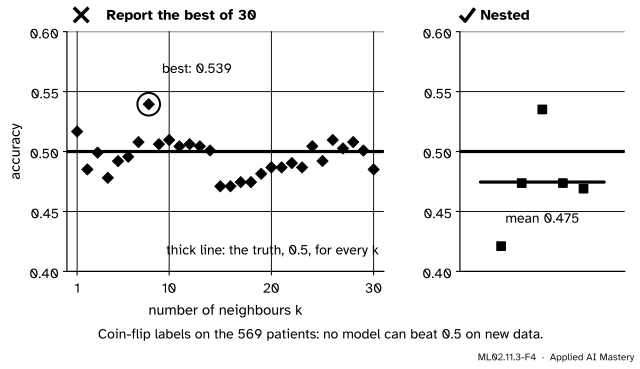
With another shuffle the \(k\)-NN gap is smaller still, and still undecided. Last, the luck of the winner. Give the patients coin-flip labels, so that no model can beat one half on new data, and tune \(k\) over 30 values.
from sklearn.model_selection import GridSearchCV, StratifiedKFold, cross_val_scorey_coin = np.random.default_rng(2).integers(0, 2, len(X)) # labels unrelated to Xinner = StratifiedKFold(5, shuffle=True, random_state=0)ks =list(range(1, 31))tuning = np.array([cross_val_score(make_pipeline(StandardScaler(), KNeighborsClassifier(k)), X, y_coin, cv=inner).mean()for k in ks])print(f"30 settings: mean {tuning.mean():.3f}, best {tuning.max():.3f} at k = {ks[tuning.argmax()]}")search = GridSearchCV(make_pipeline(StandardScaler(), KNeighborsClassifier()), {"kneighborsclassifier__n_neighbors": ks}, cv=inner)nested = cross_val_score(search, X, y_coin, cv=StratifiedKFold(5, shuffle=True, random_state=1))print(f"nested cross-validation of the whole search: {nested.mean():.3f}")
30 settings: mean 0.496, best 0.539 at k = 8
nested cross-validation of the whole search: 0.475
Averaged over the 30 settings the score is \(0.496\), honest. The best is \(0.539\), nearly four points of skill that do not exist. Scoring the whole search, tuning included, on outer folds it never saw gives \(0.475\): no skill, as it should be.
Explore
This module’s interactive, the model line-up, is in lesson 1. Pick the Blobs + noise feature preset and press New sample several times. The four accuracies jump by a point or two each time, and their order changes. That jumping is the fold-to-fold variation of this lesson.
Pitfalls
ML02.11.3-F4
Wrong beside right, on labels that carry no information. The best of 30 settings claims skill; nested cross-validation, which scores the whole search, does not.
“k-NN lost 19 of 25 folds, so logistic regression is better.”
Counting wins treats the folds as independent, and they are not: the same 569 patients are scored five times over, by models trained on overlapping data. The corrected standard error says the gap of \(0.013\) is \(1.8\) errors from zero. Not decided.
“I scaled the whole table once, then cross-validated.”
Then every training fold was scaled with means and spreads that included its held-out rows. With standardising the harm is small; with feature selection or target encoding it can be large (ML01.10.2, ML02.5.3). Put every step inside the pipeline.
“I tuned all four models on these folds and report the best one’s score.”
That score is the best of many, and the best of many is flattered: on coin-flip labels it shows \(0.539\) where the truth is \(0.5\). Report the score of the whole procedure with nested cross-validation, which ML04.4 and ML04.5 treat in full, or confirm the winner on data the search never saw.
Check yourself
Recall
1. What do stratified folds keep the same in every fold?
Show answer
The share of each class, equal to its share in the whole table.
2. Why are the 25 fold differences of five repeated five-fold runs not independent?
Show answer
Training sets overlap (two in the same repeat share three of four folds) and every repeat reuses the same rows, so the differences are positively correlated.
3. Write the corrected standard error for \(J\) differences from \(k\)-fold splits.
Show answer
\(\text{SE}_\text{corr} = s\sqrt{1/J + 1/(k-1)}\), where \(s\) is the standard deviation of the differences.
4. When is a difference between two models “decided” in this lesson?
Show answer
When the mean difference is more than two corrected standard errors from zero.
5. Why is the best of 30 tuned scores too optimistic, and what fixes it?
Show answer
It is the luckiest of 30 noisy estimates on these folds. Nested cross-validation scores the whole tuning procedure on outer folds it never saw.
Exercises
1.★ Ten repeats of ten-fold cross-validation give 100 differences with standard deviation \(0.02\) and mean \(0.006\). Compute the naive and the corrected standard errors and say whether the difference is decided.
Show solution
Naive: \(0.02/\sqrt{100} = 0.002\), so the mean is \(3\) standard errors out. Corrected, with \(k = 10\): \(0.02\sqrt{1/100 + 1/9} = 0.02\sqrt{0.0100 + 0.1111} = 0.02 \times 0.348 = 0.0070\). The mean is \(0.006/0.0070 = 0.86\) standard errors from zero: not decided.
2.★★ With \(k = 5\), does the corrected standard error keep shrinking as \(J\) grows? Find the limit of \(\text{SE}_\text{corr}/s\) as \(J \to \infty\) and say what it means for running more repeats.
Show solution
\(\text{SE}_\text{corr}/s = \sqrt{1/J + 1/4}\). As \(J\) grows, \(1/J \to 0\) and the ratio tends to \(\sqrt{1/4} = 0.5\). At \(J = 25\) it is already \(0.539\), and at \(J = 100\) it is \(\sqrt{0.26} = 0.510\). Beyond a few repeats, more repeats barely help: the shared part \(\rho\sigma^2\) of Result 1 does not average away. Only more data, which lowers \(\sigma^2\) itself, sharpens the comparison.
3.★★★ Use Result 1 to show that if the differences were independent (\(\rho = 0\)), the naive standard error would be right on average in the sense \(\E[s^2/J] = \text{Var}(\bar{d})\). Then show that for \(\rho > 0\) the naive variance \(s^2/J\) is too small on average, by finding the ratio \(\text{Var}(\bar{d}) / \E[s^2/J]\).
Show solution
By Result 2, \({\E[s^2]} = {(1 - \rho)\sigma^2}\), so \(\E[s^2/J] = {(1 - \rho)\sigma^2/J}\). With \(\rho = 0\) this is \(\sigma^2/J\), and Result 1 gives \(\text{Var}(\bar{d}) = \sigma^2/J\) too. In general
which exceeds 1 whenever \(\rho > 0\) and grows with \(J\). With \(J = 25\) and \(\rho = 0.2\) the true variance is \(1 + 25 \times 0.25 = 7.25\) times the naive one on average.
Summary card
Same folds, paired differences, a corrected error bar: and a gap smaller than two of them decides nothing.
ML02.11.3-F1
Naive bar clear, corrected bar touching zero.
Fair: same repeated stratified folds for every model; every step inside the pipeline.
Correlated folds:\({\text{Var}(\bar{d}) = \rho\sigma^2 + (1-\rho)\sigma^2/J}\) and \({\E[s^2] = (1-\rho)\sigma^2}\).
Corrected:\({\text{SE}_\text{corr} = s\sqrt{1/J + 1/(k-1)}}\); decided when \({\abs{\bar{d}} > 2\,\text{SE}_\text{corr}}\).
Winner’s luck: the best of many tuned scores is too high; nested CV scores the whole search.
Sources and next steps
Sources. Each was opened and checked against this lesson on 15 November 2026.
Claude Nadeau and Yoshua Bengio, Inference for the Generalization Error, NeurIPS 1999. Section 2, Lemma 1: for \(k\) variables with common variance and correlation \(\pi\), the sample variance has expectation \({\delta(1 - \pi)}\) and the mean has variance \({\delta(\pi + (1 - \pi)/k)}\). Section 3, the corrected resampled \(t\)-test: the variance of the mean estimated by \({(1/J + n_2/n_1)\hat\sigma^2}\), with \(n_1\) training and \(n_2\) test examples, from the stand-in \(\rho_0 = {n_2/(n_1 + n_2)}\).
scikit-learn 1.9, Statistical comparison of models using grid search: models scored on the same RepeatedStratifiedKFold partitions are correlated, assuming independence underestimates the variance, and the corrected_std function multiplies the variance of the differences by \(1/(kr) + n_\text{test}/n_\text{train}\).
scikit-learn 1.9 user guide, Section 3.1, Cross-validation: cross_validate, stratified \(k\)-fold and repeated \(k\)-fold, and pipelines that keep preprocessing inside each fold.
Gavin Cawley and Nicola Talbot, On Over-fitting in Model Selection and Subsequent Selection Bias in Performance Evaluation, Journal of Machine Learning Research 11 (2010), pages 2079 to 2107. Section 1: model selection must be “performed afresh every time a model is fitted to a new sample of data”, which calls for protocols such as nested cross-validation. Section 5: evaluation protocols that leave the selection outside show an optimistic bias, sometimes as large as the differences between algorithms.