Logistic regression grows into softmax regression: one score per class, the softmax turns the scores into probabilities, and the cross-entropy gradient is prediction minus one-hot label times the input. Then the K by K confusion matrix and its macro, micro and weighted averages.
ML02.10.1L2 Intermediate25 minIn review (what this means)
The maths and code on this page are checked by automated tests on every change, but an independent reader has not signed it off yet. Spot a mistake or a confusing step? Tell us.
Write softmax regression for K classes: K score vectors, the softmax, and the cross-entropy loss of one example.
Derive the gradient of the loss with respect to each score vector, (p_k - y_k) x, and run gradient descent with it.
Explain why one of the K score vectors is redundant and what fixes it.
Compute per-class precision, recall and F1 from a K by K confusion matrix, and their macro, micro and weighted averages.
The question
A spam filter answers yes or no. A triage system must choose between stroke, overdose and seizure; a digit reader between ten digits; a language model between fifty thousand words. How do we turn the one-score logistic regression of ML01.6 into a model that picks one class out of many, trains with the same gradient descent, and is judged fairly when the classes are of different sizes?
Intuition
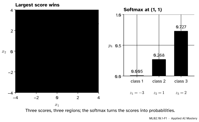
Give every class its own score. Class \(k\) gets a linear score \({z_k = \vect{w}_k \cdot \vect{x} + b_k}\), so with \(K\) classes there are \(K\) weight vectors. The class with the largest score wins its part of the plane. The softmax of ML01.6.4 then turns the \(K\) scores into \(K\) probabilities that add up to 1.
ML02.10.1-F1
Softmax regression on the three clusters of this module. Left: each class owns the region where its score is largest, and the borders are straight. Right: at the new point \((1, 1)\) the scores \({(-3, 1, 2)}\) become the probabilities \({(0.005, 0.268, 0.727)}\).
Three things in the picture carry the whole lesson. The borders are straight lines, because the border between classes \(j\) and \(k\) is where \({z_j = z_k}\), a linear equation. Every point gets a full set of probabilities, not just a winner. And the model is trained by making the probability of each example’s true class large, which is the same likelihood idea as in ML01.6.2.
Some models need none of this. A tree’s leaf can hold a majority among \(K\) classes, \(k\)-nearest neighbours can vote among \(K\) classes, and naive Bayes and LDA compare \(K\) posteriors. Logistic regression is the one model of ML01 built around two classes, so it is the one that needs extending.
Build it up
Step 1. Scores. Collect the weight vectors as the rows of a matrix \(\mat{W}\) and the biases in \(\vect{b}\). Then all \(K\) scores at once are \({\vect{z} = \mat{W}\vect{x} + \vect{b}}\).
Step 2. Probabilities. Exponentiate and normalise:
\[
\cmodel{p_k} = \frac{e^{z_k}}{\sum_{j=1}^{K} e^{z_j}} , \qquad k = 1, \dots, K .
\]
Step 3. The label as a vector. Write the true class \(c\) as a one-hot vector \(\ctruth{\vect{y}}\) with \({y_c = 1}\) and every other entry 0. For class 2 of 3 that is \({(0, 1, 0)}\).
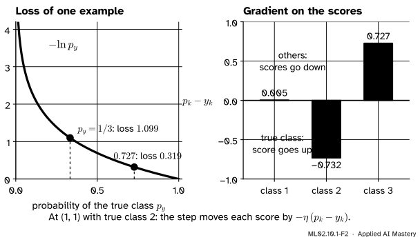
Step 4. The loss. The cross-entropy of one example is
minus the log of the probability given to the true class. Only that one term survives the sum. It is the negative log-likelihood of ML01.6.2 with \(K\) outcomes instead of two.
ML02.10.1-F2
Left: the loss is small only when the true class gets a high probability. Right: the gradient with respect to the scores is \({p_k - y_k}\). It is negative for the true class only, so a descent step raises that score and lowers all the others.
The formal statement
NoteSoftmax regression
For \(K\) classes, inputs \(\vect{x} \in \R^d\), weights \(\vect{w}_1, \dots, \vect{w}_K\) and biases \(b_1, \dots, b_K\), the model is
It is fitted by minimising the mean cross-entropy over the \(n\) training examples, and it predicts the class with the largest probability, which is the class with the largest score.
ISL calls this multinomial logistic regression with the softmax coding.
The gradient, derived. Take one example with true class \(c\). Since \({\ln p_c = z_c - \ln \sum_j e^{z_j}}\),
\[
L = -z_c + \ln \sum_{j=1}^{K} e^{z_j} .
\]
Differentiate with respect to one score \(z_k\). The first term gives \(-1\) if \({k = c}\) and \(0\) otherwise, which is \(-y_k\). The second term is a log of a sum, so its derivative is the derivative of the sum, \(e^{z_k}\), divided by the sum:
The score \(z_k\) depends on \(\vect{w}_k\) through \({z_k = \vect{w}_k \cdot \vect{x} + b_k}\), so \({\pd{z_k}{\vect{w}_k} = \vect{x}}\) and \({\pd{z_k}{b_k} = 1}\). By the chain rule,
For the mean loss over \(n\) examples, average these over the examples. This is the binary result of ML01.6.3, prediction minus label times the input, now once per class. Gradient descent updates every \(\vect{w}_k\) at once by \({-\eta}\) times its gradient.
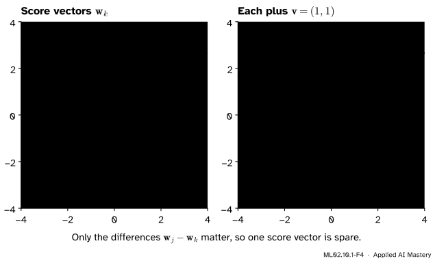
One score vector is spare. Add the same vector \(\vect{v}\) to every \(\vect{w}_k\) and the same number \(a\) to every \(b_k\). Every score grows by the same amount \({\vect{v} \cdot \vect{x} + a}\), and the softmax ignores a common shift (ML01.6.4, exercise 3). So the model has more parameters than it can use. Two ways out:
Fix \({\vect{w}_K = \vect{0}}\) and \({b_K = 0}\), and fit the other \({K - 1}\). Class \(K\) becomes the baseline, as in ISL’s equations (4.10) and (4.11). With \({K = 2}\) this is logistic regression.
Keep all \(K\) and add an L2 penalty. Among the equally good shifted solutions the penalty picks the one with \({\sum_k \vect{w}_k = \vect{0}}\) (proof below).
ML02.10.1-F4
Shifting every score vector by the same \(\vect{v}\) moves the arrows but not their differences, so the borders and the probabilities do not move.
Go deeper: why the L2 penalty makes the score vectors sum to zero
Take any solution and shift it by \(\vect{v}\). The loss does not change, and the penalty becomes \({\sum_k \norm{\vect{w}_k - \vect{v}}^2}\). Its derivative with respect to \(\vect{v}\) is \({-2\sum_k (\vect{w}_k - \vect{v})}\), which is zero at \({\vect{v} = \tfrac{1}{K}\sum_k \vect{w}_k}\), the mean of the vectors. So the penalised optimum is the shift whose mean is \(\vect{0}\), that is, \({\sum_k \vect{w}_k = \vect{0}}\). Plain gradient descent started at zero keeps this too: the gradients \({(p_k - y_k)\vect{x}}\) add up to \({(1 - 1)\vect{x} = \vect{0}}\) over the classes, so every step adds vectors that sum to zero.
The \(K\) by \(K\) confusion matrix. Row \(i\), column \(j\) counts the examples of true class \(i\) predicted as class \(j\). For class \(k\), the diagonal entry is its true positives, the rest of its column is its false positives and the rest of its row is its false negatives. Precision, recall and F1 follow as in ML01.7.2, one class at a time. Three ways combine them into one number:
macro average: the plain mean over the \(K\) classes, so every class counts the same;
weighted average: the mean weighted by each class’s number of true examples, its support;
micro average: add up the true positives, false positives and false negatives of all classes first, then compute the metric once.
In a single-label problem every mistake is one false positive (for the predicted class) and one false negative (for the true class). So the pooled false positives equal the pooled false negatives, and micro precision, micro recall and micro F1 all equal the accuracy.
Worked example
One gradient step on the three clusters. The twelve points have class means \({(-2, -1)}\), \({(2, -1)}\) and \({(0, 2)}\), and their overall mean is the origin. Start from \({\mat{W} = \mat{0}}\), \({\vect{b} = \vect{0}}\).
Step 0. Every score is 0, so every probability is \({1/3}\) and the loss of every point is \({\ln 3 = 1.099}\).
The gradient for class \(k\). Average \({(1/3 - y_{ik})\,\vect{x}_i}\) over the twelve points. The \({1/3}\) part averages to a third of the overall mean, which is \(\vect{0}\). The \(y_{ik}\) part keeps only the four points of class \(k\), giving \({\tfrac{4}{12}}\) times their mean. So
where \(\bar{\vect{x}}_k\) is the mean of class \(k\). The bias gradients are \({1/3 - 4/12 = 0}\).
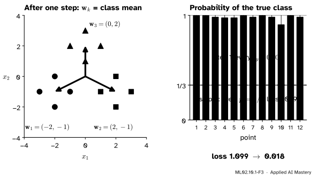
The step. With learning rate \({\eta = 3}\), chosen to keep the numbers whole, \({\vect{w}_k = 0 - 3 \cdot (-\tfrac{1}{3}\bar{\vect{x}}_k) = \bar{\vect{x}}_k}\): \({\vect{w}_1 = (-2, -1)}\), \({\vect{w}_2 = (2, -1)}\), \({\vect{w}_3 = (0, 2)}\). They sum to \(\vect{0}\), as the deeper note promised.
ML02.10.1-F3
One step from zero. Each score vector becomes its class mean, every point’s true class now has probability at least \(0.909\), and the mean loss falls from \(1.099\) to \(0.018\).
A new point. At \({\vect{x} = (1, 1)}\) the scores are \({-2 - 1 = -3}\), \({2 - 1 = 1}\) and \({0 + 2 = 2}\). The exponentials are \(0.0498\), \(2.718\) and \(7.389\), with sum \(10.157\), so
and the model predicts class 3. If the true class were class 2, the loss would be \({-\ln 0.268 = 1.318}\) and the score gradient \({\vect{p} - \vect{y} = (0.005,\ -0.732,\ 0.727)}\).
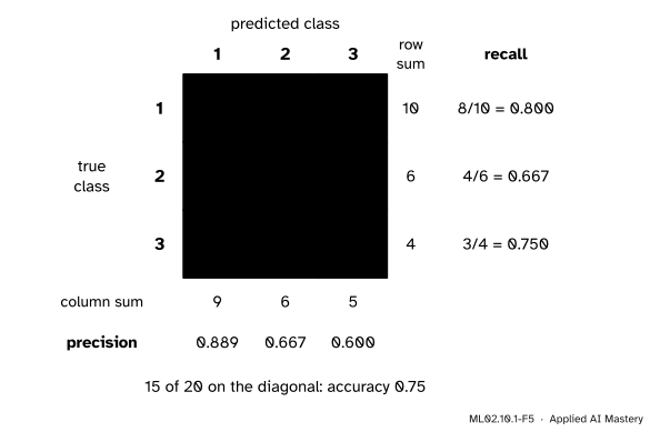
A confusion matrix by hand. Twenty test examples of three classes give this matrix.
ML02.10.1-F5
Recall runs along a row (of the true examples of a class, how many were found); precision runs down a column (of the predictions of a class, how many were right).
The F1 of each class is \({2\,TP / (2\,TP + FP + FN)}\): \({16/19 = 0.842}\), \({8/12 = 0.667}\) and \({6/9 = 0.667}\). Then
macro precision is the mean of \(0.889\), \(0.667\) and \(0.600\), which is \(0.719\); in the same way macro recall is \(0.739\) and macro F1 is \(0.725\);
weighted F1, with weights \(10\), \(6\) and \(4\) out of \(20\), is \({0.754}\), and weighted recall is \({(8 + 4 + 3)/20 = 0.75}\);
micro precision, recall and F1 are all \({15/20 = 0.75}\), the accuracy.
Weighted recall always equals the accuracy too, because each class’s recall times its share of the examples is its diagonal count divided by \(n\).
Code
First the step of the worked example, from scratch with NumPy.
import numpy as npX = np.array([[-3, -1], [-2, -2], [-2, 0], [-1, -1], [1, -1], [2, -2], [2, 0], [3, -1], [-1, 2], [0, 1], [0, 3], [1, 2]], dtype=float)y = np.repeat([0, 1, 2], 4) # classes 1, 2, 3 are 0, 1, 2 in codeY = np.eye(3)[y] # one-hot rowsdef softmax_rows(Z): E = np.exp(Z - Z.max(axis=1, keepdims=True)) # a common shift changes nothingreturn E / E.sum(axis=1, keepdims=True)def loss_and_grads(W, b, X, Y): P = softmax_rows(X @ W.T + b) loss =-np.mean(np.log(P[Y ==1])) G = (P - Y) /len(X) # dL/dz for every example and classreturn loss, G.T @ X, G.sum(axis=0) # gradients for W (K by d) and bW, b = np.zeros((3, 2)), np.zeros(3)loss0, gW, gb = loss_and_grads(W, b, X, Y)W, b = W -3* gW, b -3* gbloss1, _, _ = loss_and_grads(W, b, X, Y)p_new = softmax_rows(np.array([[1.0, 1.0]]) @ W.T + b)[0]print("loss", round(loss0, 3), "->", round(loss1, 3))print("W after one step:\n", W.round(3))print("p at (1, 1):", p_new.round(3))
loss 1.099 -> 0.018
W after one step:
 [[-2. -1.]
 [ 2. -1.]
 [-0.  2.]]
p at (1, 1): [0.005 0.268 0.727]
Now the same loop on iris: 150 flowers, 4 measurements, 3 species. scikit-learn’s LogisticRegression fits softmax regression whenever there are three or more classes, with an L2 penalty \({\tfrac{1}{2}\norm{\mat{W}}^2}\) against \(C\) times the summed loss. Dividing by \(Cn\) turns that into the mean loss plus \({\tfrac{1}{2Cn}\norm{\mat{W}}^2}\), which our loop can match.
from sklearn.datasets import load_irisfrom sklearn.linear_model import LogisticRegressionfrom sklearn.preprocessing import StandardScaleriris = load_iris()Xi = StandardScaler().fit_transform(iris.data)Yi = np.eye(3)[iris.target]lam =1/ (1.0*len(Xi)) # C = 1W, b = np.zeros((3, 4)), np.zeros(3)for step inrange(20000): _, gW, gb = loss_and_grads(W, b, Xi, Yi) W, b = W -0.5* (gW + lam * W), b -0.5* gb# a tight tolerance, so that the library's answer is as exact as our long loopmodel = LogisticRegression(C=1.0, tol=1e-10, max_iter=10000).fit(Xi, iris.target)print("largest gap to scikit-learn:", float(np.abs(W - model.coef_).max()))print("coef_ columns sum to:", model.coef_.sum(axis=0).round(12))print("correct on the training flowers:", int((model.predict(Xi) == iris.target).sum()), "of 150")
largest gap to scikit-learn: 2.9919449984205926e-07
coef_ columns sum to: [-0. -0. -0. -0.]
correct on the training flowers: 146 of 150
Last, the averages of the hand-worked confusion matrix, against precision_recall_fscore_support.
   macro: precision 0.719  recall 0.739  F1 0.725
weighted: precision 0.764  recall 0.750  F1 0.754
   micro: precision 0.750  recall 0.750  F1 0.750
Explore
This module’s interactive, the reduction explorer, lives in the next lesson. Its softmax mode trains this lesson’s model live on three draggable clusters, beside the one-vs-rest and one-vs-one alternatives.
Pitfalls
ML02.10.1-F6
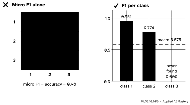
Wrong beside right. The model never predicts class 3, yet the micro-averaged F1 is \(0.90\). The per-class scores, and their macro average \(0.575\), show the failure.
“Micro-averaged F1 tells me how the model does on every class.”
For one label per example, micro F1 is the accuracy, so it is dominated by the big classes. A rare class can be missed entirely, as in the figure. Report the per-class scores, and use the macro average when every class matters equally (rare diseases, rare fraud types).
“With three classes I need three separate logistic regressions.”
That is one-vs-rest, the next lesson’s subject, and it is a different model: each of its three classifiers is trained on its own, so their probabilities need not add up to 1. Softmax regression trains the three score vectors together under one loss, and its probabilities always add up to 1.
“The fitted weights tell me how much each feature favours class \(k\).”
Only differences \({\vect{w}_j - \vect{w}_k}\) are fixed by the data. Shift every vector by the same \(\vect{v}\) and nothing changes, so a single \(\vect{w}_k\) means something only against a reference: the baseline class, or the zero mean that the L2 penalty chooses. Read coefficients as “class \(j\) against class \(k\)”.
Check yourself
Recall
1. Write the softmax probability of class \(k\) in terms of the scores.
2. What is the cross-entropy loss of one example whose true class is \(c\)?
Show answer
\({L = -\ln p_c}\): minus the log of the probability the model gives the true class.
3. What is the gradient of that loss with respect to \(\vect{w}_k\)?
Show answer
\({(p_k - y_k)\,\vect{x}}\), where \(y_k\) is the one-hot label: 1 for the true class, 0 otherwise.
4. Why is one of the \(K\) score vectors redundant?
Show answer
Adding the same vector to every \(\vect{w}_k\) adds the same amount to every score, and the softmax ignores a common shift. So one vector can be fixed at zero, or a penalty can pick the solution whose vectors sum to zero.
5. In a single-label problem, why do micro precision, micro recall and accuracy agree?
Show answer
Each mistake is one false positive and one false negative, so the pooled counts are equal and both micro precision and micro recall equal the number correct divided by \(n\).
Exercises
1.★ Scores \({(1, 0, -1)}\) for three classes. Find the probabilities, the predicted class, and the loss if the true class is class 2.
Show solution
The exponentials are \({e^{1} = 2.718}\), \({e^{0} = 1}\) and \({e^{-1} = 0.368}\), with sum \(4.086\). So \({\vect{p} = (0.665,\ 0.245,\ 0.090)}\), the same as for \({(2, 1, 0)}\) because the scores were shifted by one. The model predicts class 1. With true class 2 the loss is \({-\ln 0.245 = 1.408}\).
2.★★ Show that softmax regression with \({K = 2}\) and \({\vect{w}_2 = \vect{0}}\), \({b_2 = 0}\) is logistic regression, and find the binary weight vector.
Show solution
With \({z_2 = 0}\), \({p_1 = e^{z_1}/(e^{z_1} + 1)}\). Divide top and bottom by \(e^{z_1}\): \({p_1 = 1/(1 + e^{-z_1}) = \sigma(z_1)}\). So class 1 is the positive class of a logistic regression with weights \(\vect{w}_1\) and bias \(b_1\). Without the baseline, the binary weights are the difference \({\vect{w}_1 - \vect{w}_2}\), because only the difference of the two scores enters.
3.★★★ A confusion matrix for classes A, B, C has rows \({(50, 0, 0)}\), \({(5, 5, 0)}\) and \({(5, 0, 5)}\). Compute the accuracy, the macro F1 and the micro F1. Which number would you report to someone who cares about B and C as much as A?
Show solution
There are 70 examples and \({50 + 5 + 5 = 60}\) on the diagonal, so the accuracy and the micro F1 are \({60/70 = 0.857}\). Class A: \({TP = 50}\), \({FP = 10}\), \({FN = 0}\), so \({F1 = 100/110 = 0.909}\). Class B: \({TP = 5}\), \({FP = 0}\), \({FN = 5}\), so \({F1 = 10/15 = 0.667}\), and class C is the same, \({0.667}\). Macro F1 is \({(0.909 + 0.667 + 0.667)/3 = 0.747}\). Report the per-class F1 and the macro average: half of B and half of C are missed, which the accuracy hides.
Summary card
One score per class; softmax makes them probabilities; the gradient is \((\vect{p} - \vect{y})\,\vect{x}\).
Redundancy. Only differences of score vectors matter: fix one, or let L2 make them sum to 0.
Averages. Macro: mean over classes. Weighted: by support. Micro: pooled counts, equal to accuracy.
Sources and next steps
Sources. Each was opened and checked against this lesson on 15 November 2026.
Gareth James, Daniela Witten, Trevor Hastie and Robert Tibshirani, An Introduction to Statistical Learning, 2nd edition, Section 4.3.5: multinomial logistic regression with a baseline class, equations (4.10) to (4.12), and the softmax coding (4.13) that treats all \(K\) classes alike, with the log odds of two classes (4.14).
Stanford UFLDL tutorial, Softmax Regression: the cost and its gradient, the section on the redundant parameterisation (subtracting one vector from every parameter vector changes nothing, so one can be set to zero), and the reduction to logistic regression for two classes.
scikit-learn 1.9, LogisticRegression: with three or more classes every solver except liblinear optimises the penalised multinomial loss, and predict_proba uses the softmax; \({C = \infty}\) removes the penalty.
scikit-learn 1.9 User Guide, Section 1.12 (LogisticRegression listed as inherently multiclass) and Section 3.4.4: the definitions of macro, weighted and micro averaging (3.4.4.1), and the note that micro-averaging over all labels of a multiclass problem gives precision, recall and F1 equal to the accuracy (3.4.4.9.2).