Add the sum of squared weights to the loss and a flexible model calms down. Derive the one-feature ridge solution and its shrinkage factor, see the penalty turn into weight decay inside gradient descent, and learn why features are standardised first and the bias is left alone.
Write the ridge loss and say what each of its two parts rewards.
Derive the ridge solution for one feature and compute its shrinkage factor.
Show that the penalty turns each gradient descent update into a shrink followed by the usual step.
Explain why features are standardised before a penalised fit and why the bias is not penalised.
Fit a ridge model from scratch in NumPy and reproduce it with scikit-learn’s Ridge.
In review. The maths and code on this page are checked by automated tests on every change, but an independent reader has not signed it off yet. Spot a mistake or a confusing step? Tell us.
The question
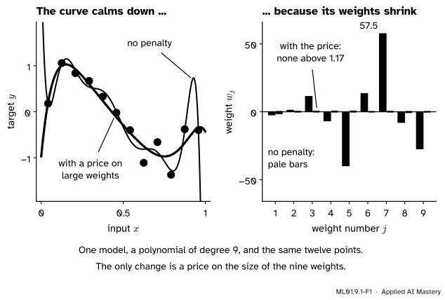
Fit a polynomial of degree 9 to twelve noisy points and it passes close to every one of them. Then, just beyond the last point, it dives to \(-10\). Its weights give it away: one is \(57.5\) and another is \(-39.8\). Could we keep the flexible model and simply charge it for using large weights? And what should the price be?
Intuition
Module ML01.8 fitted this polynomial to its dozen points and called the result overfitting. One cure was a simpler model. This lesson builds a cure that ML01.8.4 only tried: keep all nine weights, but make large ones expensive.
Why would that help? A curve that swings wildly is built from large weights of opposite sign that almost cancel. Near the training points the cancelling works. A little further on it fails, and the curve shoots away. Large weights are the mark of a model that is fitting noise.
So change what training minimises. To the fit loss, which says how badly the curve misses the points, add a second term that grows with the weights:
Adding a term like this, to hold a model back from fitting noise, is called regularisation. This form is ridge regression, and the term is the L2 penalty.
ML01.9.1-F1
The same degree-9 polynomial fitted twice to the dozen. Left: with no penalty it lunges between and beyond the last points. Right: the price cuts the largest weight from \(57.5\) to \(1.17\).
The number \(\lambda\) (lambda) is the price. At \(\lambda = 0\) nothing is charged. As \(\lambda\) grows, the weights are pushed towards zero and the curve flattens. Training does not set \(\lambda\). You do, so it is a hyperparameter (ML01.2.2). This lesson shows what the price does. Lessons 3 and 4 show how to choose it.
Build it up
Nine weights are too many to follow by hand. Start with one.
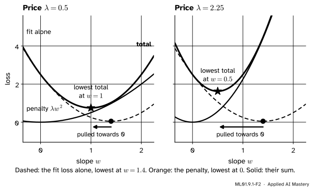
Step 1. One weight. Take the course’s four points, \(x = 1, 2, 3, 4\) and \(y = 2, 3, 5, 6\). For a line through their mean point, the fit loss is a parabola in the slope \(w\) (ML01.5.1), lowest at \(w = 1.4\).
Step 2. The penalty is a second parabola. It is \(\lambda w^2\), lowest at \(w = 0\), and it knows nothing about the data.
Step 3. Add them. The sum of two parabolas that open upward is another one. Its lowest point lies between their lowest points: the fit pulls \(w\) towards \(1.4\) and the penalty pulls it towards \(0\).
ML01.9.1-F2
The fit loss wants \(w = 1.4\). The penalty wants \(w = 0\). Their sum settles in between: at \(w = 1\) for \(\lambda = 0.5\) and at \(w = 0.5\) for \(\lambda = 2.25\).
Step 4. A higher price pulls further, but never all the way. At \(w = 0\) the penalty parabola is flat, so the first crumb of weight costs almost nothing, while it still improves the fit. Some weight is always worth having.
Step 5. The bias is not charged. The bias sets the level of the predictions. Charging for it would drag every prediction towards zero, whatever the data say.
Step 6. Every feature needs the same unit. Measure an input in minutes instead of hours and its weight becomes 60 times smaller, so the same price would hardly touch it. The cure is to standardise each feature first.
The formal statement
NoteDefinition: the ridge loss
For the model \(\hat{y}_i = w_1 x_{i1} + \dots + w_d x_{id} + b\) and a price \(\lambda \ge 0\),
are the variance of \(x\) and the covariance of \(x\) and \(y\). We also need \(s_{yy} = \frac{1}{n}\sum_i (y_i - \bar{y})^2\).
Part A: the bias. The penalty does not contain \(b\), so the slope along \(b\) is the one from ML01.4.2:
\[
\begin{aligned}
\pd{L}{b} &= \frac{2}{n}\sum_i (w x_i + b - y_i) \\
&= 2\,(w\bar{x} + b - \bar{y}) .
\end{aligned}
\]
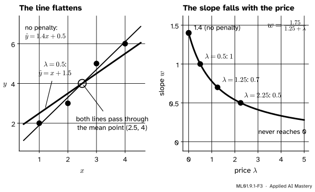
Setting it to zero gives \(b = \bar{y} - w\bar{x}\). Whatever the slope, the best line passes through the mean point \((\bar{x}, \bar{y})\).
Part B: the weight. Write \(a_i = x_i - \bar{x}\) and \(c_i = y_i - \bar{y}\) for the distances from the means. Put the \(b\) of Part A into the prediction error of example \(i\):
This shrinkage factor is \(1\) at \(\lambda = 0\) and falls towards \(0\) as \(\lambda\) grows. It is never \(0\): ridge shrinks a weight and never removes it.
Part D: units. Change the unit of the input, \(x' = c\,x\) (hours to minutes is \(c = 60\)). Then \(s_{x'x'} = c^2 s_{xx}\) and \(s_{x'y} = c\,s_{xy}\), so the new weight is \(w' = c\,s_{xy} / (c^2 s_{xx} + \lambda)\). Per old unit that is a slope of
Changing the unit by a factor \(c\) acts like changing the price to \(\lambda / c^2\). So before penalising, standardise: replace \(x_i\) by \(z_i = (x_i - \bar{x})/s\) with \(s = \sqrt{s_{xx}}\), using the mean and standard deviation of the training set (ML01.3.3). Then \(s_{zz} = 1\) whatever the unit was, and
\[
w_z = \frac{s_{zy}}{1 + \lambda} .
\]
Part E: weight decay. Gradient descent needs the slope of the ridge loss. The penalty adds \(2\lambda w_j\) to the slope \(g_j\) of the fit loss, so the update of ML01.5.2 becomes
Read it as two moves. First shrink the weight by the fixed factor \(1 - 2\eta\lambda\), a number just below 1. Then take the usual step. For this reason the L2 penalty is also called weight decay.
Go deeper: many features: the same formula with matrices
Put each example’s standardised features in a row of \(\mat{Z}\) and write \(\vect{y}_c\) for the targets minus their mean. The bias is again \(\bar{y}\), and the loss of the weights is \(\frac{1}{n}\norm{\mat{Z}\vect{w} - \vect{y}_c}^2 + \lambda\norm{\vect{w}}^2\). The gradient of the first term is \(\frac{2}{n}\mat{Z}\T(\mat{Z}\vect{w} - \vect{y}_c)\) (ML01.4.3), and that of the second is \(2\lambda\vect{w}\). Setting the sum to zero:
With one feature, \(\frac{1}{n}\mat{Z}\T\mat{Z}\) is \(s_{zz} = 1\) and the right side is \(s_{zy}\): Part D again. The \(\lambda\) on the diagonal has a second benefit. For \(\lambda > 0\) and any \(\vect{v} \ne \vect{0}\),
so the matrix sends no such \(\vect{v}\) to \(\vect{0}\), and the system has exactly one solution, even with more features than examples.
Frontier note: weight decay in deep learning
Weight decay is among the most widely used regularisers in deep learning. With plain gradient descent it is the L2 penalty, as Part E shows. With adaptive optimisers such as Adam the two differ, because the penalty’s slope is rescaled along with everything else. Loshchilov and Hutter (2019) showed this and proposed applying the shrink step separately: AdamW.
Worked example
Ridge on the four points, with \(\lambda = 0.5\).
The averages.\(\bar{x} = 2.5\) and \(\bar{y} = 4\).
\(x_i\)
\(y_i\)
\(x_i - \bar{x}\)
\(y_i - \bar{y}\)
\(1\)
\(2\)
\(-1.5\)
\(-2\)
\(2\)
\(3\)
\(-0.5\)
\(-1\)
\(3\)
\(5\)
\(0.5\)
\(1\)
\(4\)
\(6\)
\(1.5\)
\(2\)
The squared distances in \(x\) are \(2.25, 0.25, 0.25, 2.25\), which sum to \(5\). The products of the two distances are \(3, 0.5, 0.5, 3\), which sum to \(7\).
Left: the penalised line pivots about the mean point and flattens. Right: the slope against the price. It falls fast at first and never touches zero.
Was it worth it? The flatter line misses each point by \(0.5\), so its fit loss is \(0.25\), up from \(0.05\). But the total is lower:
Line
Fit loss
Penalty \(0.5\,w^2\)
Total
\(\hat{y} = 1.4x + 0.5\)
\(0.05\)
\(0.98\)
\(1.03\)
\(\hat{y} = x + 1.5\)
\(0.25\)
\(0.50\)
\(0.75\)
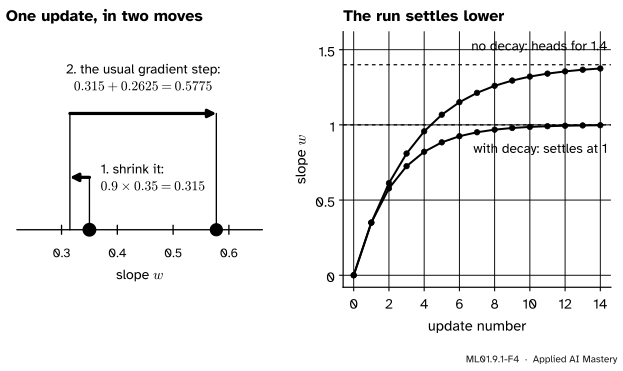
One update of weight decay. Feed the line the centred input \(x - 2.5\). By Part A its best bias is then \(\bar{y} = 4\) whatever the slope, so start gradient descent at \(w = 0\), \(b = 4\), with \(\eta = 0.1\): the bias is already right and stays. The slope of the fit loss is \(g = 2w\,s_{xx} - 2s_{xy} = 2.5w - 3.5\), and the shrink factor is \(1 - 2 \times 0.1 \times 0.5 = 0.9\).
Without the shrink, update 2 would give \(0.35 + 0.2625 = 0.6125\).
ML01.9.1-F4
Left: the second update, taken apart. Right: the whole run. With the decay, gradient descent settles on the ridge slope \(1\) instead of \(1.4\).
Code
The one-feature result, exactly as derived.
import numpy as npx = np.array([1.0, 2.0, 3.0, 4.0])y = np.array([2.0, 3.0, 5.0, 6.0])def ridge_line(x, y, lam):"""Slope and bias with the lowest ridge loss, for one feature.""" s_xx = np.mean((x - x.mean()) **2) s_xy = np.mean((x - x.mean()) * (y - y.mean())) w = s_xy / (s_xx + lam)return w, y.mean() - w * x.mean()def ridge_loss(w, b, x, y, lam):return np.mean((w * x + b - y) **2) + lam * w **2for lam in [0.0, 0.5, 1.25, 2.25]: w, b = ridge_line(x, y, lam)print(f"lam = {lam:<4}: w = {w:.3f}, b = {b:.3f}, total loss = {ridge_loss(w, b, x, y, lam):.4f}")print("total loss of the unpenalised line at lam = 0.5:", round(ridge_loss(1.4, 0.5, x, y, 0.5), 4))w =0.0for step in [1, 2]: w = (1-2*0.1*0.5) * w -0.1* (2*1.25* w -2*1.75) # shrink, then the usual stepprint(f"weight decay, update {step}: w = {w:.4f}")
lam = 0.0 : w = 1.400, b = 0.500, total loss = 0.0500
lam = 0.5 : w = 1.000, b = 1.500, total loss = 0.7500
lam = 1.25: w = 0.700, b = 2.250, total loss = 1.2750
lam = 2.25: w = 0.500, b = 2.750, total loss = 1.6250
total loss of the unpenalised line at lam = 0.5: 1.03
weight decay, update 1: w = 0.3500
weight decay, update 2: w = 0.5775
Now the dozen and the degree-9 polynomial, with twelve more examples from the same source as a validation set; of many draws, we kept one whose pictures are clear. Powers of a number between 0 and 1 all look alike (\(x^8\) and \(x^9\) are almost the same column), so the input is first re-centred to \(u = 2x - 1\), which runs from \(-1\) to \(1\). Then each of the nine powers of \(u\) is standardised with the training set’s mean and standard deviation. The solver is the matrix formula of the deeper block.
x_train = (np.arange(12) +0.5) /12# the dozen of ML01.8y_train = np.array([0.18, 1.06, 0.84, 0.67, 0.33, -0.02, -0.40, -1.11, -0.66, -1.37, -0.38, -0.40])x_val = np.array([0.11, 0.34, 0.36, 0.37, 0.43, 0.58, 0.60, 0.75, 0.85, 0.87, 0.91, 0.98])y_val = np.array([0.93, 0.76, 0.45, 1.03, 0.11, -0.21, -0.23, -1.20, -0.88, -1.14, -0.89, -0.45])def powers(x, degree=9): u =2* x -1# centre the input firstreturn np.column_stack([u ** k for k inrange(1, degree +1)])def fit_ridge(x, y, lam, degree=9):"""Standardise with this training set, then solve (Z'Z/n + lam I) w = Z'(y - mean y)/n.""" F = powers(x, degree) mu, sd = F.mean(axis=0), F.std(axis=0) Z, b, n = (F - mu) / sd, y.mean(), len(y)if lam ==0: w = np.linalg.lstsq(Z, y - b, rcond=None)[0] # plain least squareselse: w = np.linalg.solve(Z.T @ Z / n + lam * np.eye(degree), Z.T @ (y - b) / n) predict =lambda q: (powers(q, degree) - mu) / sd @ w + breturn w, predictmse =lambda predict, x, y: float(np.mean((predict(x) - y) **2))for lam in [0.0, 0.01, 10.0]: w, predict = fit_ridge(x_train, y_train, lam)print(f"lam = {lam:<5}: largest |w| = {np.abs(w).max():6.2f}, sum of squares = {np.sum(w **2):8.2f}, "f"training error = {mse(predict, x_train, y_train):.3f}, validation error = {mse(predict, x_val, y_val):.3f}")print("no penalty, prediction at x = 0.93 and x = 1:", np.round(fit_ridge(x_train, y_train, 0.0)[1](np.array([0.93, 1.0])), 2))
lam = 0.0  : largest |w| =  57.52, sum of squares =  6056.41, training error = 0.019, validation error = 1.182
lam = 0.01 : largest |w| =   1.17, sum of squares =     1.86, training error = 0.043, validation error = 0.126
lam = 10.0 : largest |w| =   0.05, sum of squares =     0.00, training error = 0.446, validation error = 0.503
no penalty, prediction at x = 0.93 and x = 1: [  0.73 -10.31]
\(\lambda\)
\(0\)
\(0.01\)
\(10\)
Largest weight
\(57.52\)
\(1.17\)
\(0.05\)
Training error
\(0.019\)
\(0.043\)
\(0.446\)
Validation error
\(1.182\)
\(0.126\)
\(0.503\)
A small price costs a little training error and cuts the validation error ninefold. A huge price flattens the curve into the mean and both errors are bad: underfitting. Without the penalty the curve climbs to \(0.73\) at \(x = 0.93\), where the points nearby sit at \(-0.4\), and reaches \(-10.31\) at \(x = 1\).
Weight decay reaches the same weights, and so does scikit-learn’s Ridge, whose alpha is \(n\lambda\) because it charges against a sum of squared errors.
from sklearn.linear_model import Ridgefrom sklearn.pipeline import make_pipelinefrom sklearn.preprocessing import PolynomialFeatures, StandardScalerlam, lr =0.01, 0.1F = powers(x_train)Z = (F - F.mean(axis=0)) / F.std(axis=0)w_gd = np.zeros(9)for _ inrange(20_000): g =2* Z.T @ (Z @ w_gd + y_train.mean() - y_train) /12# slope of the fit loss w_gd = (1-2* lr * lam) * w_gd - lr * g # shrink, then the usual stepu_train = (2* x_train -1).reshape(-1, 1)library = make_pipeline(PolynomialFeatures(9, include_bias=False), StandardScaler(), Ridge(alpha=12* lam)).fit(u_train, y_train)w_solve = fit_ridge(x_train, y_train, lam)[0]print("formula: ", np.round(w_solve, 3))print("weight decay:", np.round(w_gd, 3))print("scikit-learn:", np.round(library[-1].coef_, 3), " bias", round(float(library[-1].intercept_), 3))
ML01.8.4 tried a price of \(0.001\) on the powers of \(x\) itself. That number does not carry over: a price has no meaning apart from the features it is charged on.
Explore
This module’s interactive, the penalty explorer, lives in the next lesson, where you can slide \(\lambda\) and watch the nine weights and the validation error respond.
Pitfalls
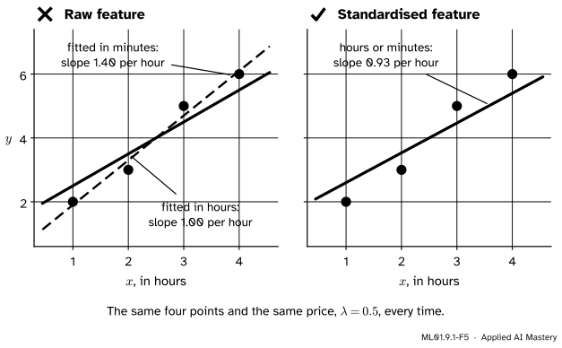
ML01.9.1-F5
Wrong beside right. Left: on the raw feature, the answer depends on the unit. Fitted in minutes, the line is hardly penalised at all. Right: after standardising, hours and minutes give the same line.
“The penalty treats all features alike, so the raw features will do.”
It treats all weights alike, and a weight’s size depends on its feature’s unit. With \(\lambda = 0.5\) the four points get the slope \(1.00\) per hour when \(x\) is in hours and \(1.40\) per hour when \(x\) is in minutes: by Part D the price has become \(0.5/3600\). Standardise first, with the training set’s mean and standard deviation. Then both give \(0.93\) per hour.
“Penalise every parameter, the bias too.”
Then the answer depends on where zero happens to be for the target. Add \(100\) to the four targets and penalise \(b\) like \(w\): the best “line” becomes \(\hat{y} = 23.07x + 30.89\), which uses a steep slope to climb towards the data because the bias is taxed. With \(b\) left free the line is \(\hat{y} = x + 101.5\), the old line moved up by \(100\).
“With a large enough price, ridge switches a feature off.”
The shrinkage factor \(s_{xx}/(s_{xx} + \lambda)\) is positive for every finite \(\lambda\). At \(\lambda = 10\) the nine weights are tiny, the largest \(0.05\), and none is zero. Removing features is the job of a different penalty, in the next lesson.
“A price of 0.01 means the same in every library.”
Conventions differ. Our \(\lambda\) is added to a mean squared error; Ridge(alpha=...) adds to a sum, so alpha is \(n\lambda\). LogisticRegression(C=...) uses an inverse: by ML01.6.3 its penalty is \(\frac{1}{2nC}w^2\), so \(\lambda = 1/(2nC)\). Check the formula before copying a number.
Check yourself
Recall
1. Write the ridge loss for a line \(\hat{y} = wx + b\).
Show answer
\(L = \frac{1}{n}\sum_i (wx_i + b - y_i)^2 + \lambda w^2\). The bias is not penalised.
2. What is the ridge slope for one feature, and what is its shrinkage factor?
Show answer
\(w = s_{xy}/(s_{xx} + \lambda)\). Compared with the least-squares slope it is multiplied by \(s_{xx}/(s_{xx} + \lambda)\).
3. With one feature, can the ridge weight be exactly zero when the least-squares weight is not?
Show answer
No. The shrinkage factor is positive for every finite \(\lambda\), so the weight shrinks and never reaches zero.
4. How does the penalty change one gradient descent update?
Show answer
The weight is first multiplied by \(1 - 2\eta\lambda\), then the usual step \(-\eta g\) is taken. This is weight decay.
5. Why are features standardised before a penalised fit?
Show answer
A weight’s size depends on its feature’s unit: changing the unit by a factor \(c\) acts like changing the price to \(\lambda/c^2\). After standardising, every feature has variance 1 and is charged at the same rate.
Exercises
1.★ Fit ridge to the four points with \(\lambda = 2.25\). Give the slope, the bias and the shrinkage factor.
Show solution
\(w = 1.75/(1.25 + 2.25) = 1.75/3.5 = 0.5\) and \(b = 4 - 0.5 \times 2.5 = 2.75\). The shrinkage factor is \(1.25/3.5 = 0.357\): the slope is \(0.357 \times 1.4 = 0.5\).
2.★★ Which price halves the least-squares slope of one feature? Answer in general, then for the four points, then for a standardised feature.
Show solution
The factor must be one half: \(s_{xx}/{(s_{xx} + \lambda)} = \tfrac12\), so \(2s_{xx} = s_{xx} + \lambda\) and \(\lambda = s_{xx}\). The price that halves the slope equals the variance of the feature. For the four points \(\lambda = 1.25\), and indeed \(1.75/(1.25 + 1.25) = 0.7 = 1.4/2\). A standardised feature has variance 1, so \(\lambda = 1\).
3.★★★ For one centred feature, show that gradient descent with weight decay settles on the ridge slope, and find the learning rates for which it converges.
Show solution
The slope of the fit loss is \(g = 2w\,s_{xx} - 2s_{xy}\), so one update is
so \(w^* = s_{xy}/{(s_{xx} + \lambda)}\): the ridge slope. Subtracting \(w^*\) from both sides of the update gives \(w - w^* \leftarrow m\,{(w - w^*)}\) with \(m = 1 - 2\eta\,(s_{xx} + \lambda)\). By ML01.5.3 the distance shrinks exactly when \(-1 < m < 1\), that is \(0 < \eta < 1/(s_{xx} + \lambda)\). For the four points with \(\lambda = 0.5\) the limit is \(1/1.75 = 0.571\), and \(\eta = 0.1\) gives \(m = 0.65\).
Summary card
Ridge adds a price on squared weights: the fit gets a little worse and the curve much calmer.
Standardise first. Then \(w_z = s_{zy}/(1 + \lambda)\), in any unit.
By hand. Four points, \(\lambda = 0.5\): slope \(1.4 \to 1\), bias \(0.5 \to 1.5\).
The dozen.\(\lambda = 0.01\): largest weight \(57.5 \to 1.17\), validation error \(1.18 \to 0.13\).
Sources and next steps
Sources. Each was opened and checked against this lesson on 12 November 2026.
Trevor Hastie, Robert Tibshirani and Jerome Friedman, The Elements of Statistical Learning, 2nd edition (free PDF from the authors), Section 3.4.1. Defines ridge regression (equation 3.41) on a sum of squared errors, so their \(\lambda\) is \(n\) times ours. States that a wildly large positive coefficient can be cancelled by a large negative one on a correlated variable, that the solutions are not equivariant under scaling of the inputs, “so one normally standardizes the inputs”, and that the intercept is left out of the penalty so that the fit does not depend on the origin chosen for the target. Gives the matrix solution (3.44) and, for orthonormal inputs, the factor \(1/(1 + \lambda)\).
Ian Goodfellow, Yoshua Bengio and Aaron Courville, Deep Learning, MIT Press, 2016, Sections 7.1 and 7.1.1. Says that the biases are typically left unregularised, names the L2 penalty weight decay and ridge regression, and writes the update as a multiplicative shrink followed by the usual gradient step (equation 7.5). Their penalty is \(\frac{\alpha}{2}w^2\), so their \(\alpha\) is our \(2\lambda\).
Tengyu Ma and Andrew Ng, CS229 Lecture Notes, Stanford University, Section 9.1. Defines the regularised loss \(J(\theta) + \lambda R(\theta)\) (equation 9.1), derives the weight-decay form of the update (9.2), and calls weight decay the most common regulariser in deep learning.
scikit-learn 1.9 User Guide, Section 1.1.2, Ridge regression and classification. Gives the objective of Ridge as \(\norm{\mat{X}\vect{w} - \vect{y}}^2 + \alpha\norm{\vect{w}}^2\), a sum, which is why alpha is \(n\lambda\).
Ilya Loshchilov and Frank Hutter, Decoupled Weight Decay Regularization, ICLR 2019. The abstract states that L2 regularisation and weight decay are equivalent for standard stochastic gradient descent but not for adaptive gradient algorithms such as Adam. Algorithm 2 names the decoupled method AdamW.