Neighbours can predict a number as well as a label: average the targets of the k nearest. Then count what a prediction costs when the model is the data itself, and see by simulation why neighbours stop being near when there are many features.
Predict a number with k-nearest-neighbour regression by averaging the targets of the k nearest examples, by hand and in NumPy.
Explain why k-nearest-neighbour regression cannot predict beyond the range of its training targets.
Count the numbers stored and the arithmetic done for one brute-force prediction, and compare both with a fitted line.
Derive the edge length a neighbourhood needs in order to hold a given share of evenly spread data in d dimensions.
Describe from a simulation how the nearest and the farthest distance compare as the number of features grows.
In review. The maths and code on this page are checked by automated tests on every change, but an independent reader has not signed it off yet. Spot a mistake or a confusing step? Tell us.
The question
So far the neighbours have voted for a label. Can they also predict a number, such as a price? And two questions every method must face. What does one prediction cost, when the “model” is the whole training set? Does “nearest” still mean anything when an example has a thousand features instead of two?
From the last lesson
1. Why does a feature recorded in large numbers dominate Euclidean distance?
Show answer
The distance adds squared differences across features without regard to units, so the feature with the largest differences supplies almost all of the sum.
2. How is a feature standardised, and where do the two numbers come from?
Show answer
\({z = (x - \mu) / \sigma}\), with the mean \(\mu\) and the standard deviation \(\sigma\) computed from the training set only.
Intuition
To predict a number, keep everything from lesson 2 except the last step. Find the \(k\) nearest stored examples and, instead of counting labels, average their targets. That is \(k\)-nearest-neighbour regression.
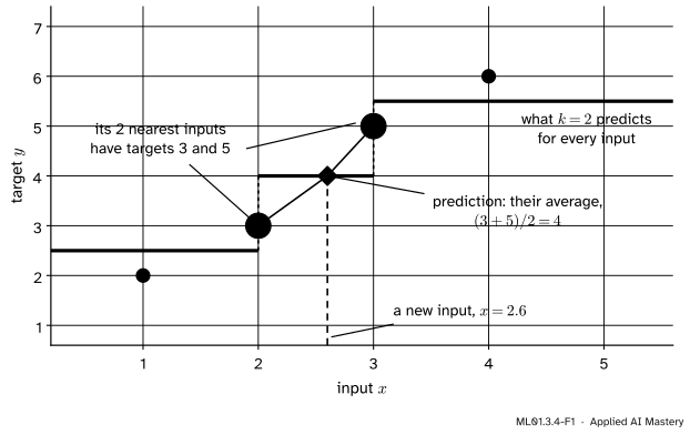
The picture uses the course’s four points, \({x = 1, 2, 3, 4}\) with targets \({y = 2, 3, 5, 6}\). With one feature, “distance” is just how far apart two inputs are on the horizontal axis.
ML01.3.4-F1
\(k\)-NN regression with \({k = 2}\). For the new input \({x = 2.6}\) the two nearest stored inputs are \(3\) and \(2\). The prediction is the average of their targets, \(4\). Doing the same for every input gives the staircase.
The prediction is flat wherever the set of neighbours stays the same, and it jumps where one neighbour is swapped for another. No slope was learned. As before, the data are the model.
Build it up
Step 1. Find the \(k\) nearest, exactly as for classification. Distances, sort, keep \(k\). Everything lesson 3 said about scaling the features still applies.
Step 2. Average instead of voting. Add the \(k\) targets and divide by \(k\).
Step 3. The same dial. With \({k = 1}\) the staircase passes through every training point. With \({k = n}\) it is a flat line at the mean of all the targets. In between, a validation set chooses \(k\), as in lesson 2.
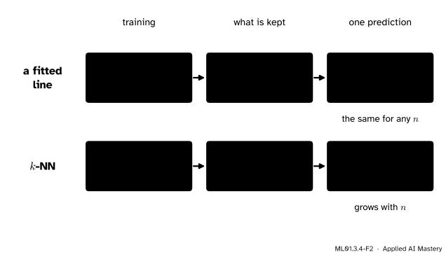
Step 4. Count what is stored and what a prediction costs. A fitted line does its work once, in training, and then keeps only its slope and intercept. \(k\)-NN does nothing in training and keeps everything.
ML01.3.4-F2
Where the work is done. A fitted line pays in training and predicts almost for nothing. \(k\)-NN pays nothing in training and pays at every prediction, more for every stored row.
To answer one query, the plain method measures the distance to all \(n\) stored examples: about \({n \times d}\) subtractions, and the same again for the next query.
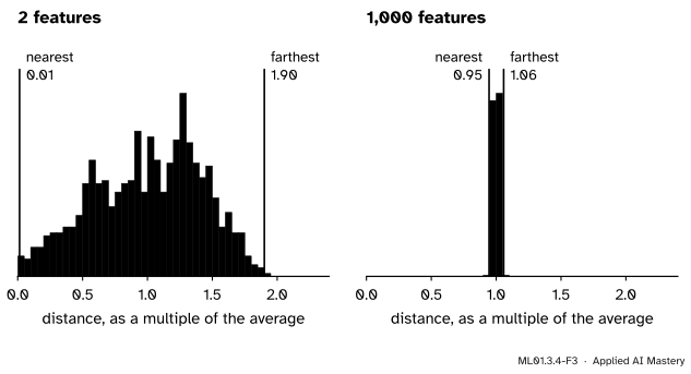
Step 5. Add features and watch “near” fade. With two features, a query has some stored points very close and others far away. That contrast is what makes the nearest neighbours special. With many features it shrinks.
ML01.3.4-F3
One query and 1,000 random points in a unit cube. Left: with 2 features the nearest point is at \(0.01\) of the average distance and the farthest at \(1.90\). Right: with 1,000 features every point is at nearly the same distance: the nearest at \(0.95\) of the average, the farthest at \(1.06\).
When every stored example is about as far away as every other, the “nearest” ones are nearest by a hair, and there is little reason to think they resemble the query more than the rest do.
The formal statement
NoteDefinition: k-nearest-neighbour regression
With \(N_k(\vect{x})\) the set of indices of the \(k\) training examples closest to the query \(\vect{x}\), the prediction is the mean of their targets:
Fact 1: the two ends of the dial. If \({k = 1}\) and the query is a training input \(\vect{x}_i\), its nearest neighbour is itself, so \({\hat{y}(\vect{x}_i) = y_i}\) and the training error is \(0\) (provided no two examples share the same inputs). If \({k = n}\), every example is a neighbour of every query, and \({\hat{y}(\vect{x}) = \frac{1}{n} \sum_i y_i = \bar{y}}\), the mean target.
Fact 2: the prediction never leaves the range of the training targets. Let \(y_{\max}\) be the largest training target. Every \({y_i \le y_{\max}}\), so
The same argument with the smallest target gives \({\hat{y}(\vect{x}) \ge y_{\min}}\). So \(k\)-NN regression cannot follow a trend beyond its data. With one feature, every query past the largest input picks the same \(k\) neighbours (exercise 3).
Fact 3: what is stored and what one prediction costs. The training set is \(n\) examples of \(d\) features: \({n \times d}\) numbers are kept, plus \(n\) targets. One squared distance needs \(d\) subtractions and \(d\) multiplications, and a query needs \(n\) of them: about \({n \times d}\) subtractions per prediction. A fitted line keeps \(d\) weights and a bias, \({d + 1}\) numbers, and predicts with \(d\) multiplications, however many examples it was trained on. With a million stored examples and 100 features, \(k\)-NN does \(10^8\) subtractions for one prediction. The line does 100 multiplications.
Fact 4: in many dimensions a neighbourhood must be wide to hold anything. Suppose the data are spread evenly through the unit cube: each of the \(d\) features runs from \(0\) to \(1\). A smaller cube with edge length \(e\) has volume \({e \times e \times \dots \times e = e^d}\), which is also the share of the data inside it. For it to hold a share \(r\),
\[
e^d = r \quad\Longrightarrow\quad e = r^{1/d} .
\]
Ask for the nearest \(1\%\) of the data, \({r = 0.01}\):
Features \(d\)
Edge needed, \({0.01^{1/d}}\)
\(1\)
\(0.01\)
\(2\)
\(0.10\)
\(3\)
\(0.22\)
\(10\)
\(0.63\)
\(100\)
\(0.95\)
On a line, \(1\%\) of the data fits in \(1\%\) of the range. With 10 features, the neighbourhood that holds \(1\%\) of the data spans \(63\%\) of the range of every feature. Such neighbours are not local. This is one face of the curse of dimensionality.
Fact 5: every added feature multiplies the data needed. With 100 points spread evenly on a line of length \(1\), neighbours are \(0.01\) apart. A grid with a point every \(0.01\) along each of \(d\) axes needs \(100^d\) points: \(10^{20}\) for \({d = 10}\). No dataset is that large, so in high dimensions every dataset is sparse.
Go deeper: why the distances bunch together
Take two random points in the unit cube, and call one coordinate of each \(U\) and \(V\), independent and evenly spread between \(0\) and \(1\). Then \({\E[U] = \tfrac12}\) and \({\E[U^2] = \int_0^1 u^2 \, du = \tfrac13}\), the same for \(V\), and independence gives \({\E[UV]} = {\E[U]\,\E[V]} = \tfrac14\). So
With \(d\) coordinates the expected squared distance is \({d / 6}\), so the square root of the average squared distance is \({\sqrt{d / 6}}\): \(0.58\) for \({d = 2}\) and \(12.9\) for \({d = 1000}\). In the simulation below, the gap between the farthest and the nearest of 1,000 points stays near \(1.4\) from \({d = 10}\) upwards, while the distances themselves keep growing.
Frontier note: how nearest-neighbour search survives in practice
Real data are not spread evenly through a cube: images and sentences occupy a small, structured part of their space. Beyer and colleagues, who proved that under broad conditions the farthest distance divided by the nearest tends to 1, also identify workloads where it does not.
Nor need the search be exhaustive. scikit-learn can index the data with a KD tree, fast below about twenty features, and approximate nearest-neighbour libraries trade a little accuracy for much more speed.
Worked example
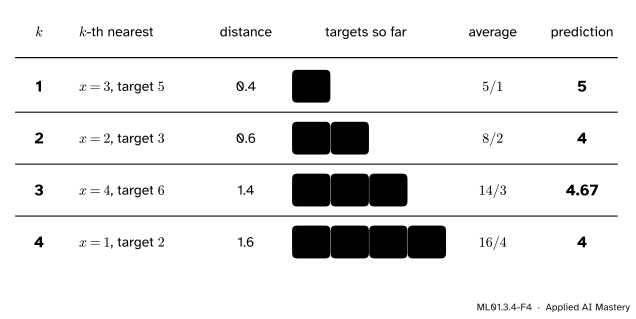
Predict the target at \({x = 2.6}\) from the four points, for every \(k\).
Step 1: the distances. From \(2.6\) to the inputs \({1, 2, 3, 4}\) the distances are \({\abs{1 - 2.6} = 1.6}\), \({\abs{2 - 2.6} = 0.6}\), \({\abs{3 - 2.6} = 0.4}\) and \({\abs{4 - 2.6} = 1.4}\).
\({k = 4}\): \({\hat{y} = (5 + 3 + 6 + 2) / 4} = 4\), the mean of all four targets, as Fact 1 says.
The least-squares line through these points, \({\hat{y} = 1.4x + 0.5}\), gives \({1.4 \times 2.6 + 0.5 = 4.14}\) here, close to the \(k\)-NN answers.
Now go outside the data. At \({x = 8}\) the two nearest inputs are \(4\) and \(3\), with targets \(6\) and \(5\), so \({k = 2}\) predicts \(5.5\), and it predicts \(5.5\) at \({x = 80}\) as well. The line predicts \({1.4 \times 8 + 0.5 = 11.7}\). By Fact 2, no \(k\) can make \(k\)-NN answer more than \(6\).
Code
From scratch: the distances are absolute differences, and the vote is replaced by a mean.
import numpy as npx = np.array([1.0, 2.0, 3.0, 4.0])y = np.array([2.0, 3.0, 5.0, 6.0])def knn_regress(x, y, query, k): order = np.argsort(np.abs(x - query), kind="stable") # nearest firstreturn y[order[:k]].mean()print(" k at x = 2.6 at x = 8")for k in [1, 2, 3, 4]:print(f" {k}{knn_regress(x, y, 2.6, k):9.2f}{knn_regress(x, y, 8.0, k):8.2f}")print(f"line {1.4*2.6+0.5:9.2f}{1.4*8+0.5:8.2f}")
  k   at x = 2.6   at x = 8
  1        5.00       6.00
  2        4.00       5.50
  3        4.67       4.67
  4        4.00       4.00
line        4.14      11.70
Now scikit-learn’s KNeighborsRegressor, on the same four points and then on real data: the diabetes dataset, 442 patients with 10 measurements each and a target measuring how far the disease has progressed a year later. The features are standardised inside a pipeline, as lesson 3 requires.
from sklearn.datasets import load_diabetesfrom sklearn.linear_model import LinearRegressionfrom sklearn.model_selection import train_test_splitfrom sklearn.neighbors import KNeighborsRegressorfrom sklearn.pipeline import make_pipelinefrom sklearn.preprocessing import StandardScalertiny = KNeighborsRegressor(n_neighbors=2).fit(x.reshape(-1, 1), y)print("four points, k = 2, at x = 2.6 and x = 8:", tiny.predict([[2.6], [8.0]]))data = load_diabetes(scaled=False)X_train, X_test, y_train, y_test = train_test_split(data.data, data.target, test_size=0.2, random_state=0)def mse(model, X, target):return np.mean((model.predict(X) - target) **2)results = {}for k in [1, 5, 20, 100, len(X_train)]: model = make_pipeline(StandardScaler(), KNeighborsRegressor(n_neighbors=k)).fit(X_train, y_train) results[k] = (mse(model, X_train, y_train), mse(model, X_test, y_test))print(f"k = {k:3d} training MSE {results[k][0]:5.0f} test MSE {results[k][1]:5.0f}")line = LinearRegression().fit(X_train, y_train)baseline = np.mean((y_train.mean() - y_test) **2)print(f"a fitted line training MSE {mse(line, X_train, y_train):5.0f} test MSE {mse(line, X_test, y_test):5.0f}")print(f"always predict the training mean test MSE {baseline:5.0f}")
four points, k = 2, at x = 2.6 and x = 8: [4.  5.5]
k =   1   training MSE     0   test MSE  8104
k =   5   training MSE  2317   test MSE  4195
k =  20   training MSE  2882   test MSE  3432
k = 100   training MSE  3549   test MSE  3584
k = 353   training MSE  6131   test MSE  5135
a fitted line       training MSE  2735   test MSE  3424
always predict the training mean                 test MSE  5135
The dial behaves as Fact 1 says. At \({k = 1}\) the training error is \(0\) and the test error, \(8104\), is the worst in the table: worse than \(5135\), the error of always predicting the training mean. At \({k = 353}\), \(k\)-NN is that mean. In between, \({k = 20}\) gives \(3432\), level with the fitted line’s \(3424\). (To pick \(k\) for real, use a validation set.)
Next, the cost of answering the 89 test patients.
n, d = X_train.shapem =len(X_test)print(f"the line keeps {line.coef_.size +1} numbers; k-NN keeps {X_train.size} feature values and {n} targets")print(f"k-NN, one query: {n} distances = {n * d:,} subtractions. All {m} queries: {m * n * d:,}")print(f"the line, one query: {d} multiplications. All {m} queries: {m * d}")print(f"a million stored examples with 100 features: {10**6*100:,} subtractions for one query")
the line keeps 11 numbers; k-NN keeps 3530 feature values and 353 targets
k-NN, one query: 353 distances = 3,530 subtractions.  All 89 queries: 314,170
the line, one query: 10 multiplications.  All 89 queries: 890
a million stored examples with 100 features: 100,000,000 subtractions for one query
Last, the simulation behind the histogram figure: 1,000 random points in the unit cube, 100 random queries, and the average nearest and farthest distance.
def distance_spread(d, n=1000, queries=100, seed=0): rng = np.random.default_rng(seed) points, ask = rng.random((n, d)), rng.random((queries, d))# squared distances for every query and point, from |a - b|^2 = |a|^2 - 2 a.b + |b|^2 squared = (ask **2).sum(axis=1)[:, None] -2* ask @ points.T + (points **2).sum(axis=1)[None, :] dist = np.sqrt(np.maximum(squared, 0))return dist.min(axis=1).mean(), dist.max(axis=1).mean(), (dist.min(axis=1) / dist.max(axis=1)).mean()print(" d nearest farthest nearest/farthest edge for 1%")spread = {}for d in [1, 2, 3, 10, 100, 1000]: spread[d] = distance_spread(d)print(f"{d:4d}{spread[d][0]:7.3f}{spread[d][1]:7.3f}{spread[d][2]:16.3f}{0.01** (1/ d):11.2f}")
With 2 features the nearest point is at about \(0.02\) of the distance of the farthest. With 10 features the ratio is already \(0.26\), with 100 it is \(0.70\), and with 1,000 it is \(0.89\): the “nearest” neighbour is only about a tenth closer than the farthest point.
Explore
The neighbour explorer in lesson 2 classifies, but its dial is this lesson’s dial too. On the noisy data, push \(k\) to its largest value: the vote ties everywhere, whatever the query, as the staircase goes flat when \({k = n}\). Each time you move the query, the explorer measures the distance to every stored point again. With 40 points that is instant. Fact 3 says what happens with 40 million.
Pitfalls
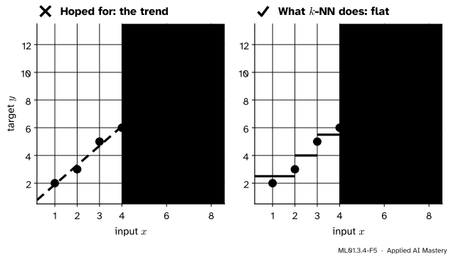
ML01.3.4-F5
Wrong beside right. Beyond the data a fitted line carries the trend on. \(k\)-NN has no trend to carry: it repeats the average of the last few targets for ever.
“The targets are rising, so \(k\)-NN will predict higher values further out.”
By Fact 2 its prediction is an average of stored targets and cannot exceed the largest of them. At \({x = 8}\) the line says \(11.7\) and \(k\)-NN with \({k = 2}\) says \(5.5\). Neither is sure to be right, but only the line can express “the trend continues”. Use \(k\)-NN to fill in between examples, not to forecast beyond them.
“There is no training, so \(k\)-NN is the cheap option.”
The cost has moved, not gone. Every prediction touches every stored example, and all of them must be kept in memory. For a model that answers millions of queries, slow training and fast answers are the better deal.
“More features mean more information, so they can only help.”
Every feature adds a term to every distance, whether or not it has anything to do with the target. Add enough of them and all the distances look alike, as the simulation showed. \(k\)-NN works best with a few well-chosen, scaled features, and needs far more data as their number grows.
Check yourself
Recall
1. How does \(k\)-nearest-neighbour regression make a prediction?
Show answer
It returns the mean target of the \(k\) training examples closest to the query.
2. What does it predict when \(k\) equals the number of training examples?
Show answer
The mean of all the training targets, for every query.
3. Why can it not predict a value larger than the largest training target?
Show answer
It is an average of training targets, and an average never exceeds its largest value.
4. What does brute-force \(k\)-NN keep, and what does it compute for one prediction?
Show answer
It keeps all \(n\) training examples. For one query it computes \(n\) distances, about \({n \times d}\) subtractions and multiplications, then picks the \(k\) smallest.
5. Data are spread evenly in a 10-dimensional unit cube. What edge must a sub-cube have to hold \(1\%\) of them?
Show answer
\({0.01^{1/10} \approx 0.63}\): the neighbourhood spans \(63\%\) of the range of every feature, so “near” neighbours are not near.
Exercises
1.★ With the four points, predict the target at \({x = 1.8}\) for \({k = 1}\), \(2\) and \(3\).
Show solution
The distances from \(1.8\) to the inputs \({1, 2, 3, 4}\) are \({0.8,\ 0.2,\ 1.2,\ 2.2}\). Nearest first: \({x = 2}\) (target \(3\)), \({x = 1}\) (target \(2\)), \({x = 3}\) (target \(5\)). So \({k = 1}\) gives \(3\), \({k = 2}\) gives \({(3 + 2) / 2 = 2.5}\) and \({k = 3}\) gives \({(3 + 2 + 5) / 3 \approx 3.33}\). The line gives \({1.4 \times 1.8 + 0.5 = 3.02}\).
2.★★ (a) A system stores 2 million examples with 50 features each. How many subtractions does brute-force \(k\)-NN perform to answer 1,000 queries? At \(10^9\) a second, how long is that? (b) Data are spread evenly in a unit cube with 10 features. What share lies in a sub-cube with edge \(0.5\)? What edge is needed to hold \(10\%\)?
Show solution
(a) \({m \times n \times d} = {1000 \times 2{,}000{,}000 \times 50} = 10^{11}\) subtractions: \(100\) seconds. A fitted line would need \({1000 \times 50 = 50{,}000}\) multiplications.
(b) The share is the volume, \({0.5^{10} = 1/1024 \approx 0.001}\): a tenth of one percent. For \(10\%\), \({e = 0.1^{1/10} \approx 0.79}\).
3.★★★ A training set has one feature, with all inputs different and largest input \(x_{\max}\). Show that for every query \({x > x_{\max}}\), \(k\)-NN regression gives the same prediction, and say what it is.
Show solution
Take any query \({x > x_{\max}}\). Every training input satisfies \({x_i < x}\), so its distance from the query is \({\abs{x - x_i} = x - x_i}\). Input \(i\) is nearer than input \(l\) exactly when \({x - x_i < x - x_l}\), that is, when \({x_i > x_l}\). The query has dropped out of the comparison, so beyond \(x_{\max}\) the training inputs are always ranked in the same order, largest first.
The \(k\) nearest are therefore always the \(k\) largest training inputs, and the prediction is the mean of their targets, a constant. For the four points with \({k = 2}\) it is \({(6 + 5) / 2 = 5.5}\), at \({x = 8}\) and at \({x = 80}\) alike.
Summary card
For a number, average the neighbours. The data are the model, and that has a price.
ML01.3.4-F1
Average the nearest targets.
Rule.\({\hat{y}(\vect{x}) = \frac{1}{k} \sum_{i \in N_k(\vect{x})} y_i}\). At \({k = n}\) it is the mean target \(\bar{y}\).
Limits.\({y_{\min} \le \hat{y} \le y_{\max}}\): no extrapolation. At \({x = 8}\) the line says \(11.7\), \(k\)-NN says \(5.5\).
Cost. Keep \({n \times d}\) numbers. One prediction needs about \({n \times d}\) subtractions. A line keeps \({d + 1}\) numbers.
Many features. To hold a share \(r\) of evenly spread data needs edge \({r^{1/d}}\): \(0.63\) for \(1\%\) when \({d = 10}\).
Simulation. Nearest over farthest distance: \(0.02\) with 2 features, \(0.89\) with 1,000.
Sources and next steps
Sources. Each was opened and checked against this lesson on 12 November 2026.
scikit-learn 1.9 user guide, Sections 1.6.3 and 1.6.4. A query’s value is the mean of the values of its nearest neighbours. Brute-force query time grows as \(O[DN]\) for \(N\) samples in \(D\) dimensions, and a KD tree is very fast below about 20 dimensions but inefficient beyond.
scikit-learn 1.9 documentation, KNeighborsRegressor. The target is predicted by local interpolation of the targets of the nearest neighbours.
Trevor Hastie, Robert Tibshirani and Jerome Friedman, The Elements of Statistical Learning, 2nd edition. Equation 2.8 (Section 2.3.2) defines the \(k\)-nearest-neighbour fit as an average. Section 2.5 gives the edge length \({r^{1/p}}\) for \(p\) inputs, with \(0.63\) for \({r = 0.01}\) and ten inputs, and the count \(100^{10}\).
Kevin Beyer, Jonathan Goldstein, Raghu Ramakrishnan and Uri Shaft, When Is “Nearest Neighbor” Meaningful?, Technical Report 1377, University of Wisconsin-Madison, June 1998. Under broad conditions, as dimensionality increases, the distance to the nearest data point approaches the distance to the farthest, though not for every workload.
Stanford University, CS231n: Deep Learning for Computer Vision, course notes: Image Classification. Approximate nearest-neighbour libraries speed up retrieval at some cost in accuracy.
The diabetes data are scikit-learn’s load_diabetes(scaled=False): 442 patients, 10 features, and a target measuring disease progression one year after baseline.
Next. Module ML01.4, Linear regression as a learning algorithm, takes the opposite approach: it compresses the training set into a few numbers, and can therefore extrapolate.