A loss gives every setting of a model’s parameters one score, and training is the search for the lowest score. Run the simplest search there is, a grid, by hand and in code, and see why it cannot scale to models with many parameters.
Say what a loss function takes in and gives out, and state training as the search for its lowest value.
Compute by hand the mean squared error of a flat line and the error rate of a threshold rule.
Run a grid search over one parameter, by hand and in code, and refine it by zooming in.
Derive why the flat line with the lowest mean squared error sits at the mean of the labels.
Count the settings a grid must try for k parameters, and explain why grid search does not scale.
In review. The maths and code on this page are checked by automated tests on every change, but an independent reader has not signed it off yet. Spot a mistake or a confusing step? Tell us.
The question
Lesson 3 left the knobs unset. A flat line can sit at any height, and someone has to choose one. Suppose you had to choose by a fixed procedure, with no judgement and no luck. What would the procedure be? And would it still work for a model with a million knobs?
From the last lesson
1. What is a model, and what do its parameters do?
Show answer
A model is a family of functions of one fixed form. Its parameters pick out one member.
2. What does turning a knob change: the input, the form of the function, or the member in use?
Show answer
The member in use. The form is fixed by the model, and the input comes from the example.
Intuition
To choose between settings you must be able to compare them. So first give every setting a score. A loss is that score: one number that says how badly the model, with its knobs at a given setting, fits the examples. Zero is a perfect fit. Bigger is worse.
Once every setting has a score, “find the best member of the family” becomes “find the setting with the lowest loss”. That search is called training. The simplest search of all is to write down a list of candidate settings, score each one, and keep the lowest.
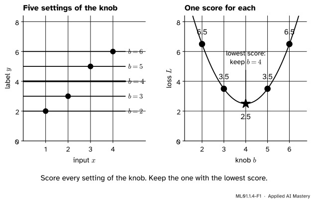
ML01.1.4-F1
Training in one picture. Left: five members of the flat-line family, one for each setting of its knob \(b\). Right: the same five settings, each with its score. The lowest point wins.
On the left are five flat lines through the four points of this course. On the right each line has become a single dot: its knob value along the bottom, its loss as its height. Training only needs the right-hand picture. The lowest dot is at \(b = 4\).
Build it up
Step 1. Score one setting. Take the flat line at \(b = 3\). It answers 3 for every input. The labels are \(2, 3, 5, 6\), so the misses, answer minus label, are \(1, 0, -2, -3\). Square each miss to get \(1, 0, 4, 9\). Take the average: \({14 / 4 = 3.5}\). This average is the mean squared error. Squaring makes a miss above and a miss below both count. It also makes one large miss cost more than small ones that add up to it: a miss of 3 costs 9, while three misses of 1 cost 3 in all. Module ML01.4 examines that choice.
Step 2. Score every setting. Do the same for any other height and you get another number. So the loss is a function of the knob, written \(L(b)\). The examples stay fixed inside it. Only the knob moves.
Step 3. Search a grid. A grid is a list of evenly spaced candidates. For \(b = 2, 3, 4, 5, 6\) the losses are \(6.5,\ 3.5,\ 2.5,\ 3.5,\ 6.5\). Keep \(b = 4\). That is a grid search, and it is a complete learning algorithm.
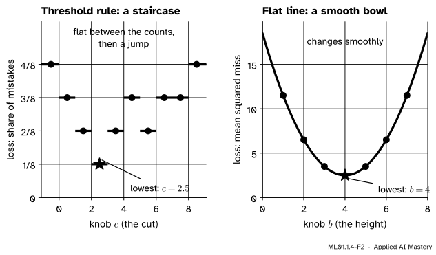
Step 4. Notice that lesson 1 did the same thing. The learner there tried ten cuts and kept the one with the fewest mistakes. Its loss was the count of mistakes, or, divided by the number of examples, the error rate.
ML01.1.4-F2
Two losses, one knob each. Left: the error rate of the threshold rule on the eight messages only changes when the cut passes a message. Right: the mean squared error of the flat line changes a little with every small turn of the knob.
Step 5. Zoom in. For the cut, ten candidates cover every way the rule can behave on the eight messages. A height can be any number, and the bottom of the bowl may fall between two candidates. The remedy is a second, finer grid around the winner of the first. The worked example does this.
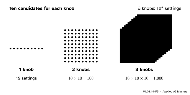
Step 6. Count the cost. With ten candidates for one knob, a grid has 10 settings to score. A model with two knobs needs every pair.
ML01.1.4-F5
Each new knob multiplies the work by ten.
Ten knobs already need ten billion settings. That is why the rest of this course looks for smarter ways to search.
The formal statement
NoteDefinition: loss and training
For a model \(f(x; \theta)\) and examples \((x_1, y_1), \dots, (x_n, y_n)\), a loss is a function \(L(\theta)\) that gives each setting of the parameters one number, small when the answers \(\hat{y}_i = f(x_i; \theta)\) are close to the labels \(y_i\). Training is finding
Read \(\argmin\) as “the setting at which \(L\) is lowest”. It names the setting, not the lowest value. This module uses two losses, and both are averages over the examples. For answers that are numbers, the mean squared error:
The sign \(\sum\) adds up over the examples. The square bracket counts: it is 1 when the statement inside is true and 0 when it is false.
Grid search. (1) Choose candidates \(\theta_1, \dots, \theta_m\). (2) Compute \(L\) at each. (3) Return the candidate with the lowest \(L\).
Result 1: the loss of a flat line is a bowl with its bottom at the mean. For \(\hat{y} = b\), expand one squared miss:
\[
(b - y_i)^2 = b^2 - 2b\,y_i + y_i^2 .
\]
Average over the examples. Neither \(b^2\) nor \(2b\) depends on \(i\), so they come out of the average. Write \(\bar{y} = \frac{1}{n} \sum_i y_i\) for the mean of the labels:
The second part does not contain \(b\). The first is a square, so it is never negative, and it is zero only when \(b = \bar{y}\). So the loss is lowest at \(b = \bar{y}\), the mean of the labels.
For our labels the mean, the mean of the squares and the loss are
Check it against Step 1: \({L(3) = 1 + 2.5 = 3.5}\).
Result 2: how close a grid gets. Let the candidates be \(h\) apart, with \(\bar{y}\) somewhere between the first and the last. Then some candidate lies within \(h/2\) of \(\bar{y}\). By Result 1 its loss is above the lowest possible by \({(b - \bar{y})^2 \le (h/2)^2}\). With \(h = 1\) that is at most \(0.25\). With \(h = 0.1\) it is at most \(0.0025\). Halving the spacing divides this bound by four.
Result 3: what a grid costs. With \(m\) candidates for each of \(k\) parameters there are \(m^k\) settings, because every choice for one knob combines with every choice for the others. Each setting needs all \(n\) examples, so the work is \(n \cdot m^k\) steps.
Go deeper: why the staircase is the harder of the two losses
For the staircase, ten candidates find the exact lowest value, so the grid is not the problem. The problem comes later, with smarter searches. Module ML01.5 finds the bottom of a bowl by feeling which way the ground slopes and stepping downhill. A staircase is flat almost everywhere. Its slope is zero, so it gives no hint about which way is down. For this reason classification models are usually trained on a smooth loss that stands in for the error rate. Module ML01.6 builds one.
Worked example
Grid search the height of the flat line by hand, in two rounds.
Round 1: candidates \(1, 3, 5, 7\). For each, write the misses \({b - y_i}\) for the labels \(2, 3, 5, 6\), square them and average.
\(b\)
Misses
Squares
Loss \(L(b)\)
1
\(-1\), \(-2\), \(-4\), \(-5\)
\(1\), \(4\), \(16\), \(25\)
\({\tfrac{46}{4} = 11.5}\)
3
\(1\), \(0\), \(-2\), \(-3\)
\(1\), \(0\), \(4\), \(9\)
\({\tfrac{14}{4} = 3.5}\)
5
\(3\), \(2\), \(0\), \(-1\)
\(9\), \(4\), \(0\), \(1\)
\({\tfrac{14}{4} = 3.5}\)
7
\(5\), \(4\), \(2\), \(1\)
\(25\), \(16\), \(4\), \(1\)
\({\tfrac{46}{4} = 11.5}\)
Two candidates tie at \(3.5\). The loss is a bowl with a single dip, so its bottom lies between them.
Round 2: candidates \(3, 3.5, 4, 4.5, 5\). Three of them are new.
\(b\)
Misses
Squares
Loss \(L(b)\)
3.5
\(1.5\), \(0.5\), \(-1.5\), \(-2.5\)
\(2.25\), \(0.25\), \(2.25\), \(6.25\)
\({\tfrac{11}{4} = 2.75}\)
4
\(2\), \(1\), \(-1\), \(-2\)
\(4\), \(1\), \(1\), \(4\)
\({\tfrac{10}{4} = 2.5}\)
4.5
\(2.5\), \(1.5\), \(-0.5\), \(-1.5\)
\(6.25\), \(2.25\), \(0.25\), \(2.25\)
\({\tfrac{11}{4} = 2.75}\)
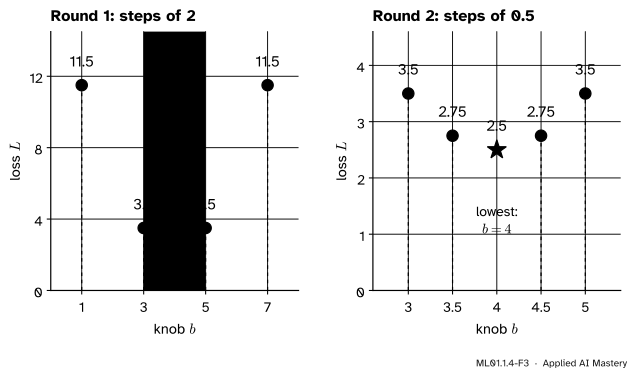
ML01.1.4-F3
Two rounds of grid search. The coarse grid finds the region. The fine grid, inside the yellow band, finds the bottom.
The winner is \(b = 4\), with loss \(2.5\). It took seven evaluations of the loss. Result 1 says the true bottom is at \(\bar{y} = 4\), so this grid landed on it exactly. That is luck. Result 2 gives what was guaranteed: with candidates \(0.5\) apart, a loss within \(0.0625\) of the lowest.
Code
From scratch: a loss, and a search that works for any loss.
ys = [2, 3, 5, 6] # the labels of the four pointsdef loss_flat(b):"""Mean squared error of the flat line y_hat = b."""returnsum((b - y) **2for y in ys) /len(ys)def grid_search(loss, candidates):"""Score every candidate. Return the one with the lowest loss, and that loss.""" best =min(candidates, key=loss)return best, loss(best)print("losses:", [loss_flat(b) for b in [2, 3, 4, 5, 6]])print("grid search keeps", grid_search(loss_flat, [2, 3, 4, 5, 6]))print("round 1:", [loss_flat(b) for b in [1, 3, 5, 7]])print("round 2:", [loss_flat(b) for b in [3, 3.5, 4, 4.5, 5]])
The same grid_search trains lesson 1’s spam rule. Only the loss changes.
marks = [0, 1, 2, 5, 3, 4, 6, 8]spam = [0, 0, 0, 0, 1, 1, 1, 1]def loss_cut(c):"""Error rate: the share of the eight messages that the cut c gets wrong."""returnsum((x > c) != (y ==1) for x, y inzip(marks, spam)) /len(marks)cuts = [k -0.5for k inrange(10)]print("grid search keeps", grid_search(loss_cut, cuts))
grid search keeps (2.5, 0.125)
Now zoom in on real data. The labels of scikit-learn’s diabetes dataset are 442 numbers between 25 and 346. Which single number, used as the answer for every patient, has the lowest loss?
import numpy as npfrom sklearn.datasets import load_diabetestarget = load_diabetes().target # 442 patients, one label eachdef loss_real(b):returnfloat(np.mean((b - target) **2))low, high, evaluations =0.0, 400.0, 0for step in [50, 5, 0.5, 0.05]: candidates = np.arange(low, high + step /2, step) best, value = grid_search(loss_real, candidates) evaluations +=len(candidates)print(f"step {step:5}: {len(candidates):2d} candidates, best b = {best:.2f}, loss {value:.3f}") low, high = best - step, best + step # the next grid surrounds this winnerprint("evaluations:", evaluations, " the mean of the labels:", round(float(target.mean()), 3))
step    50:  9 candidates, best b = 150.00, loss 5934.437
step     5: 21 candidates, best b = 150.00, loss 5934.437
step   0.5: 21 candidates, best b = 152.00, loss 5929.903
step  0.05: 21 candidates, best b = 152.15, loss 5929.885
evaluations: 72   the mean of the labels: 152.133
Four rounds and 72 evaluations bring the grid to \(152.15\). A single grid with steps of \(0.05\) over the whole range would have needed 8,001. The mean of the labels is \(152.133\), as Result 1 predicts.
The library version of grid search is scipy.optimize.brute.
from scipy import optimizefound = optimize.brute(lambda p: loss_flat(p[0]), ranges=(slice(0, 8.25, 0.25),), finish=None)print("scipy's grid search:", found, " the mean of the labels:", np.mean(ys))for knobs in [1, 2, 3, 10, 20]: seconds =10** knobs /1e9# ten candidates a knob, a billion losses a secondprint(f"{knobs:2d} knobs: {10** knobs:.0e} settings, {seconds:.0e} seconds")print("20 knobs, in years:", round(10**20/1e9/ (365.25*24*3600)))
scipy's grid search: 4.0   the mean of the labels: 4.0
 1 knobs: 1e+01 settings, 1e-08 seconds
 2 knobs: 1e+02 settings, 1e-07 seconds
 3 knobs: 1e+03 settings, 1e-06 seconds
10 knobs: 1e+10 settings, 1e+01 seconds
20 knobs: 1e+20 settings, 1e+11 seconds
20 knobs, in years: 3169
Explore
This module’s interactive, Rule versus learner, is in lesson 1. Press Step there to watch a grid search one candidate at a time. The bars under the number line are the loss of every cut.
Pitfalls
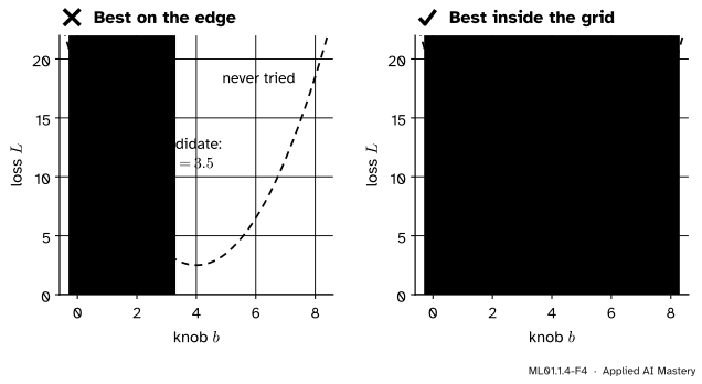
ML01.1.4-F4
Wrong beside right. A winner on the edge of the grid says the loss was still falling when the grid ran out.
“The best candidate on my grid is the best setting.”
It is only the best of those you tried. Search the heights \(0, 1, 2, 3\) and the winner is \(b = 3\), with loss \(3.5\). The bottom, at \(b = 4\), was never on the list. A winner on the edge of the grid is a warning. Widen the grid until the winner has a worse candidate on each side.
“The lowest loss gives the best model for new data.”
The loss here is measured on the same examples that chose the knobs. It tells you how well the model fits those examples, and nothing yet about examples it has not seen. Module ML01.2 is about that gap.
“With a fast enough computer, a grid will do.”
Ten candidates for each of 20 knobs make \(10^{20}\) settings. At a billion losses a second that takes about 3,169 years. Models in later courses have millions of knobs. Speed does not rescue grid search. Only a better search does.
“There is one correct loss.”
A loss is a choice, and it decides what “best” means. Score the flat line by the average size of its misses, without squaring, and every height from 3 to 5 is equally good. Exercise 3 works this out.
Check yourself
Recall
1. What does a loss function take in, and what does it give out?
Show answer
It takes a setting of the parameters and gives one number: how badly the model with that setting fits the examples. The examples are fixed inside it.
2. In terms of the loss, what is training?
Show answer
The search for the parameter setting with the lowest loss: \({\theta^\star = \argmin_\theta L(\theta)}\).
3. What are the three steps of a grid search?
Show answer
Choose a list of candidate settings, compute the loss at each, and return the candidate with the lowest loss.
4. Which flat line has the lowest mean squared error?
Show answer
The one at the mean of the labels, \(b = \bar{y}\), because \({L(b) = (b - \bar{y})^2}\) plus a part that does not contain \(b\).
5. Why does grid search fail for models with many parameters?
Show answer
With \(m\) candidates for each of \(k\) parameters there are \(m^k\) settings to score. That number grows too fast: ten candidates and 20 parameters already give \(10^{20}\).
Exercises
1.★ (a) Compute the loss of the flat line at \(b = 6\) by hand and check it with Result 1. (b) What is the error rate of the cut \(c = 4.5\) on the eight messages of lesson 1?
Show solution
(a) The misses are \({6 - 2 = 4}\), \({6 - 3 = 3}\), \({6 - 5 = 1}\) and \({6 - 6 = 0}\). Their squares are \(16, 9, 1, 0\), which sum to 26, so \({L(6) = 26/4 = 6.5}\). Result 1 gives \({(6 - 4)^2 + 2.5 = 6.5}\).
(b) The cut \(4.5\) flags the counts \(5, 6, 8\). The normal message with 5 marks is flagged, and the spam with 3 and 4 marks is let through: 3 mistakes. The error rate is \({3/8 = 0.375}\).
2.★★ Freeze the slope of a line at \(w = 1\), so that the family is \({\hat{y} = x + b}\) with one knob. On the four points, grid search \(b = 0, 1, 2, 3\) by hand. Then zoom in. Use Result 1 to say where the exact bottom is.
Show solution
The answers are \({x_i + b}\), so the misses are \({x_i + b - y_i = b - g_i}\), where the gap \({g_i = y_i - x_i}\) takes the values \(1, 1, 2, 2\).
A tie between \(1\) and \(2\), so try \(1.5\): the misses are \(0.5, 0.5, -0.5, -0.5\) and the loss is \(0.25\).
The misses have the form \({b - g_i}\), which is the flat line’s loss with \(g_i\) in place of \(y_i\). Result 1 then puts the bottom at the mean of the \(g_i\), which is \({(1 + 1 + 2 + 2)/4 = 1.5}\). The loss there is
3.★★★ Change the loss of the flat line to the mean absolute miss, \({\frac{1}{n} \sum_i \abs{b - y_i}}\). Compute it for \(b = 2, 3, 4, 5, 6\). Then show that every \(b\) from 3 to 5 has the same loss. What does that say about the choice of loss?
Show solution
At \(b = 2\) the sizes of the misses are \(0, 1, 3, 4\), with mean \({8/4 = 2}\). At \(b = 3\) they are \(1, 0, 2, 3\), mean \(1.5\). At \(b = 4\): \(2, 1, 1, 2\), mean \(1.5\). At \(b = 5\): \(3, 2, 0, 1\), mean \(1.5\). At \(b = 6\): \(4, 3, 1, 0\), mean \(2\).
Now take any \(b\) with \({3 \le b \le 5}\). It is at or above the labels 2 and 3, and at or below the labels 5 and 6. So \({\abs{b - 2} = b - 2}\), \({\abs{b - 3} = b - 3}\), \({\abs{b - 5} = 5 - b}\) and \({\abs{b - 6} = 6 - b}\). Their sum is
because the \(b\)’s cancel. The loss is \({6/4 = 1.5}\) for every such \(b\).
With squares there is one best height, \(b = 4\). With absolute values a whole stretch of heights ties for best. The examples and the family are the same. Only the loss changed. The loss is part of the problem you pose, and different losses can crown different winners.
Summary card
A loss scores every setting of the knobs. Training keeps the lowest.
ML01.1.4-F1
Score every setting, keep the lowest.
Loss. One number for each setting \(\theta\), with the examples fixed: \(L(\theta)\).
Grid search. List candidates, score each, keep the lowest. Zoom in to refine.
Flat line.\({L(b) = (b - \bar{y})^2 + \text{constant}}\), lowest at the mean \(\bar{y}\). Here \({L(b) = (b - 4)^2 + 2.5}\).
Cost.\(m\) candidates for each of \(k\) knobs: \(m^k\) settings.
Sources and next steps
Sources. Each was opened and checked against this lesson on 12 November 2026.
Simon J. D. Prince, Understanding Deep Learning, MIT Press, 2023 (free PDF, dated 8 February 2026). Section 2.1 treats the loss as a function of the parameters and training as finding the parameters that minimise it (equation 2.3). Section 2.2.2 assigns “a numerical value to each choice of parameters”, and Section 2.2.3 calls the process of minimising it model fitting, training or learning.
Marc Peter Deisenroth, A. Aldo Faisal and Cheng Soon Ong, Mathematics for Machine Learning, Cambridge University Press, 2020 (free PDF). Section 8.2.2 defines a loss function, takes its average over the training examples (equation 8.6) and gives the squared loss as an example (equation 8.7, with the factor \(1/N\) used here).
Tengyu Ma and Andrew Ng, CS229 Lecture Notes, Stanford University. Chapter 1 (page 10) defines a cost function that measures, for each value of the parameters, how close the predictions are to the targets, and then looks for a search procedure to minimise it. Their cost is half a sum of squares, where this course uses the mean.
SciPy, scipy.optimize.brute. It computes the function’s value at each point of a grid, and with finish=None returns the grid point with the lowest value.
Next. The next module, ML01.2, on the course page, asks an awkward question. The loss was measured on the same examples that chose the knobs. How well will the chosen member do on examples it has never seen?