With several features, every prediction is a row of a table times a column of weights: X times w. Derive the normal equations, solve them by hand for six flats and with NumPy’s lstsq, see how a column of ones carries the bias, and learn why X transpose X should not be inverted.
Write the predictions of a linear model with several features as the product X w, with a column of ones for the bias.
Derive the normal equations from the partial derivatives of the mean squared error.
Build and solve the normal equations by hand for a small dataset with two features.
Fit a linear model with numpy.linalg.lstsq and with scikit-learn, and check that the residuals are perpendicular to every column.
Explain why solving beats inverting, and what happens when columns are dependent or nearly so.
In review. The maths and code on this page are checked by automated tests on every change, but an independent reader has not signed it off yet. Spot a mistake or a confusing step? Tell us.
The question
Rent depends on more than the number of rooms. Where the flat is matters too. A line through one feature cannot use that. Does the exact solution of the last lesson survive with two features, or two hundred? It does, and it shrinks to one line of algebra. The product at its centre, a table of data times a column of weights, is also the product that a layer of a neural network computes.
From the last lesson
1. Give the slope and the intercept of the least-squares line.
Show answer
\(w = s_{xy}/s_x^2\), the covariance of \(x\) and \(y\) over the variance of \(x\), and \(b = {\bar{y} - w\bar{x}}\).
2. What do the two equations \(\pd{L}{b} = 0\) and \(\pd{L}{w} = 0\) say about the residuals?
Show answer
They sum to zero, \(\sum_i r_i = 0\), and so do the residuals times the inputs, \(\sum_i r_i x_i = 0\).
Intuition
Here are six invented flats. Each has two features: its number of rooms, and whether it is in the city centre (\(1\)) or not (\(0\)). The target is the monthly rent in hundreds.
Flat
Rooms \(x_1\)
Central \(x_2\)
Rent \(y\)
A
\(3\)
\(0\)
\(8\)
B
\(4\)
\(0\)
\(8\)
C
\(5\)
\(0\)
\(11\)
D
\(1\)
\(1\)
\(7\)
E
\(2\)
\(1\)
\(11\)
F
\(3\)
\(1\)
\(12\)
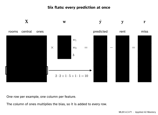
The model gives each feature its own weight and adds a bias: \(\hat{y} = {w_1 x_1 + w_2 x_2 + b}\). Now one small trick. Give every flat a third feature that is always \(1\). Then the bias is the weight of that feature, \(\hat{y} = {w_1 x_1 + w_2 x_2 + b \cdot 1}\), and a prediction is one row of the table multiplied, entry by entry, with the weights.
ML01.4.3-F1
The table as a matrix. \(\mat{X}\) holds the features and a column of ones. Multiplying it by the weights \(\vect{w}\) gives all six predictions, and subtracting the rents gives the residuals. The weights shown are the best ones, found below.
All six predictions together are the matrix \(\mat{X}\) times the vector \(\vect{w}\). With that, the last lesson can be said again in one line that holds for any number of features.
Build it up
Step 1. One prediction is a row times the weights. Flat E has the row \((2, 1, 1)\). With the weights \((2, 5, 1)\) its prediction is \(2 \cdot 2 + 1 \cdot 5 + 1 \cdot 1 = 10\).
Step 2. All predictions are \(\mat{X}\vect{w}\). Stack the rows into a matrix \(\mat{X}\) with one row per example and one column per feature, the ones included. The matrix-vector product does Step 1 for every row. Here \(\mat{X}\) is \(6 \times 3\) and \(\vect{w}\) has \(3\) entries, so the product has \(6\): one prediction per flat.
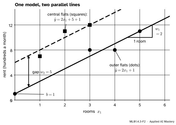
Step 3. What the model looks like. With one feature the model is a line. With two numeric features it is a flat plane above the plane of the features. Here the second feature only takes the values \(0\) and \(1\), so we see two slices of that plane: two parallel lines.
ML01.4.3-F2
The fitted model \(\hat{y} = {2x_1 + 5x_2 + 1}\). Both lines have slope \(w_1 = 2\). Being central lifts the line by \(w_2 = 5\). The bias \(b = 1\) is where the lower line meets \(x_1 = 0\).
Step 4. The loss, in the same notation. Subtract the targets from the predictions to get the vector of residuals, \(\vect{r} = \mat{X}\vect{w} - \vect{y}\). The mean squared error is the mean of its squared entries.
Step 5. One balance per column. The best line of the last lesson balanced its residuals in two ways: \(\sum_i r_i = 0\) and \(\sum_i r_i x_i = 0\). The first multiplies the residuals by the column of ones and adds. The second does the same with the column of \(x\). With more columns there is one balance for each: the residuals, multiplied by any column of \(\mat{X}\) and added up, must give zero. If not, changing that column’s weight would lower the loss.
The formal statement
NoteDefinition: the linear model in matrix form
For \(n\) examples with \(d\) features, the design matrix\(\mat{X}\) has \(n\) rows and \(d + 1\) columns: entry \(x_{ij}\) is feature \(j\) of example \(i\), and the last column is all ones. The weight vector \(\vect{w}\) has \(d + 1\) entries, the last being the bias. Then
The derivative with respect to one weight. Residual \(i\) is \(r_i = \sum_k x_{ik} w_k - y_i\). Only one term of that sum contains \(w_j\), so \(\pd{r_i}{w_j} = x_{ij}\). By the chain rule,
The sum multiplies column \(j\) of \(\mat{X}\) by \(\vect{r}\), entry by entry, and adds. That is entry \(j\) of \(\mat{X}\T\vect{r}\), since the rows of \(\mat{X}\T\) are the columns of \(\mat{X}\). Stacking the \(d + 1\) derivatives gives the gradient:
These are the normal equations: \(d + 1\) linear equations in the \(d + 1\) weights.
Check: one feature. With columns \(x\) and ones, \(\mat{X}\T\mat{X}\) has the entries \(\sum x_i^2\), \(\sum x_i\), \(\sum x_i\) and \(n\), and \(\mat{X}\T\vect{y}\) has \(\sum x_i y_i\) and \(\sum y_i\). Divided by \(n\), the two rows are \(w\,\overline{x^2} + b\bar{x} = \overline{xy}\) and \(w\bar{x} + b = \bar{y}\): the two equations of the last lesson. For the four points they read \(30w + 10b = 47\) and \(10w + 4b = 16\), and \(w = 1.4\), \(b = 0.5\) satisfies both.
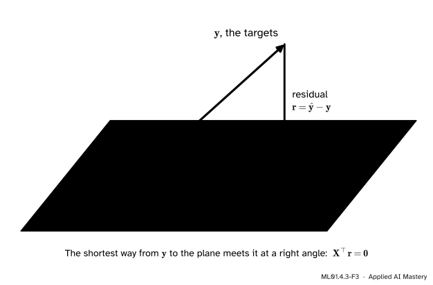
The picture. The normal equations say \(\mat{X}\T\vect{r} = \vect{0}\): the residual vector has a zero dot product with every column of \(\mat{X}\), so it is perpendicular to them all. (“Normal” is an old word for perpendicular.)
ML01.4.3-F3
Least squares as geometry. As \(\vect{w}\) varies, \(\mat{X}\vect{w}\) reaches every point of a plane, but usually not \(\vect{y}\). The best \(\hat{\vect{y}}\) is the point of the plane nearest to \(\vect{y}\), where the residual meets the plane at a right angle.
When is the answer unique? When no column of \(\mat{X}\) can be built from the others, that is, when the columns are independent. Suppose \(\mat{X}\T\mat{X}\vect{v} = \vect{0}\) for some vector \(\vect{v}\). Multiply on the left by \(\vect{v}\T\):
so \(\mat{X}\vect{v} = \vect{0}\). With independent columns that forces \(\vect{v} = \vect{0}\). So \(\mat{X}\T\mat{X}\) sends only the zero vector to zero, which makes it invertible (module M02.7), and the normal equations have exactly one solution, written on paper as \(\vect{w} = (\mat{X}\T\mat{X})^{-1}\mat{X}\T\vect{y}\). If the columns are dependent, many weight vectors give the same predictions, and all are solutions.
Go deeper: why a solution of the normal equations is the minimum
Let \(\vect{w}\) solve the normal equations, with residual \(\vect{r}\), so \(\mat{X}\T\vect{r} = \vect{0}\). Take any other weights \(\vect{w} + \vect{v}\). Their residual is \({\mat{X}(\vect{w} + \vect{v})} - \vect{y} = \vect{r} + \mat{X}\vect{v}\), and its squared length is
No change of the weights can lower the loss. Equality needs \(\mat{X}\vect{v} = \vect{0}\), which leaves the predictions unchanged. So every solution of the normal equations is a minimum. This is Pythagoras: \(\vect{r}\) and \(\mat{X}\vect{v}\) are the perpendicular sides of a right triangle.
Worked example
Fit the six flats by hand.
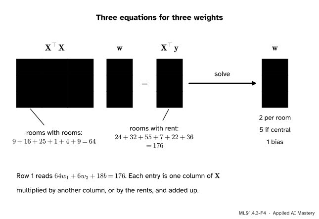
Build the equations. Each entry of \(\mat{X}\T\mat{X}\) is one column of \(\mat{X}\) multiplied by another and added up. The columns are rooms \((3, 4, 5, 1, 2, 3)\), central \((0, 0, 0, 1, 1, 1)\) and ones.
rooms with central: \(1 + 2 + 3 = 6\), and rooms with ones: \(18\)
central with central: \(3\), central with ones: \(3\), ones with ones: \(6\)
Each entry of \(\mat{X}\T\vect{y}\) is a column multiplied by the rents \((8, 8, 11, 7, 11, 12)\): rooms give \(24 + 32 + 55 + 7 + 22 + 36 = 176\), central gives \(7 + 11 + 12 = 30\), and ones give \(57\).
ML01.4.3-F4
The normal equations for the six flats: sums of products on each side, then three equations solved for three weights.
Eliminate \(w_2\) twice. (C) minus (B) gives \(12 w_1 + 3b = 27\), that is \(4 w_1 + b = 9\). (A) minus twice (B) gives \(52 w_1 + 12 b = 116\), that is \(13 w_1 + 3b = 29\). Subtract three times the first from the second: \(13 w_1 - 12 w_1 = 29 - 27\), so \(w_1 = 2\). Then \(b = 9 - 8 = 1\), and (B) gives \(12 + 3 w_2 + 3 = 30\), so \(w_2 = 5\).
Read and check. The model is \(\hat{y} = {2x_1 + 5x_2 + 1}\). The predictions are \(7, 9, 11, 8, 10, 12\) and the residuals \(-1, 1, 0, 1, -1, 0\). Against each column, leaving out the products that are zero:
In practice nobody forms \(\mat{X}\T\mat{X}\). np.linalg.lstsq takes \(\mat{X}\) and \(\vect{y}\) and returns the least-squares weights. scikit-learn adds the bias itself, so it gets the features without the column of ones.
The same lines handle a real table. scikit-learn’s diabetes dataset has 442 patients and 10 features, and its target measures how the disease progressed over a year.
from sklearn.datasets import load_diabetesdata = load_diabetes()A = np.column_stack([data.data, np.ones(len(data.target))])weights = np.linalg.lstsq(A, data.target, rcond=None)[0]sk = LinearRegression().fit(data.data, data.target)print("shape of the design matrix:", A.shape)print("largest gap between lstsq and scikit-learn:", f"{np.abs(weights[:-1] - sk.coef_).max():.0e}")print(f"MSE of the fit: {np.mean((A @ weights - data.target) **2):.1f}")
shape of the design matrix: (442, 11)
largest gap between lstsq and scikit-learn: 3e-12
MSE of the fit: 2859.7
Now the reason not to invert. Two columns that are nearly copies of each other make the problem delicate. The condition number measures how delicate: roughly, how much rounding errors can be magnified. Forming \(\mat{X}\T\mat{X}\) squares it.
rng = np.random.default_rng(0)a = rng.normal(size=50)twin = a +1e-7* rng.normal(size=50) # nearly a copy of the first columnZ = np.column_stack([a, twin, np.ones(50)])truth = np.array([1.0, 2.0, 3.0])t = Z @ truth # targets with no noise, so the right answer is knownby_inverse = np.linalg.inv(Z.T @ Z) @ Z.T @ tby_lstsq = np.linalg.lstsq(Z, t, rcond=None)[0]print(f"condition number of Z: {np.linalg.cond(Z):.0e} of Z^T Z: {np.linalg.cond(Z.T @ Z):.0e}")print(f"largest error with the inverse: {np.abs(by_inverse - truth).max():.0e}")print(f"largest error with lstsq: {np.abs(by_lstsq - truth).max():.0e}")
condition number of Z: 2e+07   of Z^T Z: 3e+14
largest error with the inverse: 3e-02
largest error with lstsq:       6e-10
The printed digits vary from machine to machine, because each rounds in its own order. The condition number goes from about \(10^7\) to about \(10^{14}\). The weights from the inverse are wrong in the first to third decimal place, depending on the machine, while those from lstsq are right to eight or nine. When one column is an exact multiple of another there is no inverse at all:
D = np.column_stack([rooms, 2* rooms, central, np.ones(6)]) # rooms, and the same thing in half-roomstry: np.linalg.inv(D.T @ D)print("an inverse came back, but it means nothing")except np.linalg.LinAlgError:print("no inverse: D^T D is singular")w_min, _, rank, _ = np.linalg.lstsq(D, rent, rcond=None)print("lstsq weights:", tidy(w_min), " rank:", rank, " predictions:", tidy(D @ w_min))
no inverse: D^T D is singular
lstsq weights: [0.4 0.8 5.  1. ]  rank: 3  predictions: [ 7.  9. 11.  8. 10. 12.]
lstsq still answers. Of all the weight vectors that fit equally well it returns the shortest: \(0.4\) per room plus \(0.8\) per half-room, that is \(0.4 + 2 \cdot 0.8 = 2\) per room, as before.
Explore
The line fitter of lesson 1 fits one feature, so its design matrix has two columns: the \(x\) of each point and a one. Drag all four points to the same \(x\) and the read-out reports that there is no single best line: the two columns have become dependent.
Pitfalls
ML01.4.3-F5
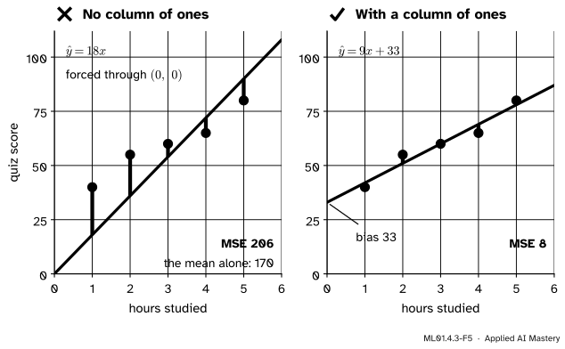
Wrong beside right, on the study table of course P01 (hours \(2, 4, 5, 1, 3\), scores \(55, 65, 80, 40, 60\)). With no column of ones the model has no bias, and its line must pass through the origin.
“np.linalg.lstsq(x, y) fits a line.”
It fits exactly the columns it is given. Pass only the hours, as one column, and the model is \(\hat{y} = wx\), a line through the origin: here \(\hat{y} = 18x\), with a loss of \(206\). Always guessing the mean score gives \(170\). With the column of ones the fit is \(\hat{y} = {9x + 33}\), with a loss of \(8\).
“The formula is \((\mat{X}\T\mat{X})^{-1}\mat{X}\T\vect{y}\), so the code is inv(X.T @ X) @ X.T @ y.”
The formula is for paper. In code the inverse is never needed: a linear system is solved directly (module M02.6), and the inverse does not even exist when columns are dependent. Worse, forming \(\mat{X}\T\mat{X}\) squares the condition number, so even solve(X.T @ X, X.T @ y) loses about twice as many digits as it has to when columns are nearly dependent. lstsq works on \(\mat{X}\) itself, and so does scikit-learn’s LinearRegression.
“More features can only help, even more features than examples.”
With more columns than rows, the columns cannot be independent. Then infinitely many weight vectors share the lowest loss, usually zero: a perfect fit of the training data. They disagree about new examples, and the training loss cannot say which to trust (modules ML01.8 and ML01.9).
Check yourself
Recall
1. What are the rows and the columns of the design matrix \(\mat{X}\)?
Show answer
One row per example and one column per feature, plus a column of ones.
2. How does the bias enter the product \(\mat{X}\vect{w}\)?
Show answer
As the weight of the column of ones. Every row multiplies it by \(1\), so it is added to every prediction.
4. In words, what does \(\mat{X}\T\vect{r} = \vect{0}\) say about the residuals of the best fit?
Show answer
The residual vector is perpendicular to every column of \(\mat{X}\): multiplied by any column and added up, the residuals give zero. For the column of ones, they sum to zero.
5. Give two reasons to call lstsq instead of inverting \(\mat{X}\T\mat{X}\).
Show answer
Forming \(\mat{X}\T\mat{X}\) squares the condition number and so loses accuracy, and the inverse does not exist when columns are dependent, while lstsq still returns a least-squares answer.
Exercises
1.★ For the four points \(x = (1, 2, 3, 4)\), \(y = (2, 3, 5, 6)\), write the design matrix, compute \(\mat{X}\T\mat{X}\) and \(\mat{X}\T\vect{y}\), and solve the normal equations.
Show solution
The rows of \(\mat{X}\) are \((1, 1)\), \((2, 1)\), \((3, 1)\), \((4, 1)\): an input, then a one. Then \(x\) with \(x\) gives \(1 + 4 + 9 + 16 = 30\), \(x\) with ones \(10\), and ones with ones \(4\). On the other side, \(x\) with \(y\) gives \(2 + 6 + 15 + 24 = 47\) and ones with \(y\) gives \(16\). So
\[
\begin{aligned}
30 w + 10 b &= 47, \\
10 w + 4 b &= 16 .
\end{aligned}
\]
The second gives \(b = {4 - 2.5 w}\). Substituting, \(30w + 40 - 25w = 47\), so \(5w = 7\), \(w = 1.4\) and \(b = 4 - 3.5 = 0.5\): the line of the last lesson.
2.★★ A seventh flat has \(2\) rooms, is not central, and costs \(5\). Without solving anything again, show that adding it to the data leaves the weights \((2, 5, 1)\) unchanged.
Show solution
The model predicts \(2 \cdot 2 + 5 \cdot 0 + 1 = 5\) for the new flat, so its residual is \(0\).
The weights \((2, 5, 1)\) solve the normal equations when \(\mat{X}\T\vect{r} = \vect{0}\). Each entry of \(\mat{X}\T\vect{r}\) is a sum over the examples of a feature value times a residual. The six old terms add up to zero, and the new flat adds a term with residual \(0\). So \(\mat{X}\T\vect{r}\) is still zero for the seven flats.
The columns are still independent, as they already were in the first six rows, so the normal equations have one solution, \((2, 5, 1)\). An example that the model already predicts exactly does not move the fit.
3.★★★ Show that if two weight vectors \(\vect{w}\) and \(\vect{w}'\) both satisfy the normal equations, they make the same predictions, even when \(\mat{X}\T\mat{X}\) has no inverse. Then check it on the design with the columns rooms, twice rooms, central and ones, for the weights \((2, 0, 5, 1)\), \((0, 1, 5, 1)\) and \((0.4, 0.8, 5, 1)\). Which is the shortest?
Show solution
Subtract the two sets of normal equations: \({\mat{X}\T\mat{X}(\vect{w} - \vect{w}')} = {\mat{X}\T\vect{y} - \mat{X}\T\vect{y}} = \vect{0}\). Call \(\vect{v} = {\vect{w} - \vect{w}'}\) and multiply on the left by \(\vect{v}\T\):
So \(\mat{X}\vect{v} = \vect{0}\), that is \(\mat{X}\vect{w} = \mat{X}\vect{w}'\). No inverse was used.
For the check, the first two columns contribute \((w_1 + 2 w_2)\) times rooms. The three weight vectors give \(2 + 0 = 2\), \(0 + 2 = 2\) and \(0.4 + 1.6 = 2\), and they share the other two weights. So all three predict \(2\) per room, \(5\) if central, plus \(1\): the fit of the worked example.
Their squared lengths are \(4 + 0 + 25 + 1 = 30\), \(0 + 1 + 25 + 1 = 27\) and \(0.16 + 0.64 + 25 + 1 = 26.8\). The third is the shortest: the one lstsq returned.
Summary card
Every prediction is a row of the table times the weights, and the best weights solve one matrix equation.
ML01.4.3-F1
A table times a column of weights.
Model.\(\hat{\vect{y}} = \mat{X}\vect{w}\), with a column of ones in \(\mat{X}\) for the bias.
Gradient.\(\nabla L = \frac{2}{n}\,\mat{X}\T{(\mat{X}\vect{w} - \vect{y})}\).
Normal equations.\(\mat{X}\T\mat{X}\,\vect{w} = \mat{X}\T\vect{y}\), the same as \(\mat{X}\T\vect{r} = \vect{0}\): the residuals are perpendicular to every column.
Unique when the columns of \(\mat{X}\) are independent.
In code.np.linalg.lstsq(X, y, rcond=None). Do not invert \(\mat{X}\T\mat{X}\).
Sources and next steps
Sources. Each was opened and checked against this lesson on 12 November 2026.
Tengyu Ma and Andrew Ng, CS229 Lecture Notes, Stanford University. Chapter 1 sets \(x_0 = 1\) for the intercept term. Section 1.2.2 defines the design matrix, derives the gradient \(\mat{X}\T\mat{X}\theta - \mat{X}\T\vect{y}\) of their cost (which has a factor \(\tfrac12\) and no \(\tfrac1n\)) and the normal equations, and notes that the closed form assumes \(\mat{X}\T\mat{X}\) is invertible.
Gilbert Strang, Projection matrices and least squares, MIT OpenCourseWare 18.06SC, lecture summary. Fits a line to three points through \(A\T A\hat{\vect{x}} = A\T\vect{b}\), notes that the error is perpendicular to the columns of \(A\), and proves that \(A\T A\) is invertible when the columns are independent.
NumPy 2.5 reference, numpy.linalg.lstsq. The function minimises the Euclidean norm of \(\vect{b} - A\vect{x}\), and “if there are multiple minimizing solutions, the one with the smallest 2-norm” is returned. Its example fits a line with a column of ones.
scikit-learn 1.9, User Guide, Section 1.1.1 and LinearRegression. The solution “is computed using the singular value decomposition of X”, through scipy.linalg.lstsq, and nearly dependent columns make the estimate highly sensitive to errors in the targets.
Aston Zhang, Zachary Lipton, Mu Li and Alexander Smola, Dive into Deep Learning, Section 3.1.1.3. Folds the bias into the weights “by appending a column to the design matrix consisting of all 1s”.