import numpy as np

def true_curve(x):
    return np.sin(2 * np.pi * x)

def inputs(n):
    return (np.arange(n) + 0.5) / n

def poly(degree):  # features 1, x, ..., x^degree
    return lambda x: np.column_stack([x ** k for k in range(degree + 1)])

def wave(x):  # features 1 and sin(2 pi x)
    return np.column_stack([np.ones_like(x), np.sin(2 * np.pi * x)])

def least_squares(A, Y):
    W, *_ = np.linalg.lstsq(A, Y, rcond=None)
    return W

def ridge(A, Y, penalty):
    """Mean squared error plus penalty * (sum of squared weights), on standardised features.
    The first column of A is the column of ones. Its weight, the bias, is not penalised."""
    F = A[:, 1:]
    mean, spread = F.mean(axis=0), F.std(axis=0)
    Z = (F - mean) / spread
    n, d = Z.shape
    V = np.linalg.solve(Z.T @ Z / n + penalty * np.eye(d), Z.T @ (Y - Y.mean(axis=0)) / n)
    W = V / spread[:, None]  # back to weights on the raw features
    return np.vstack([Y.mean(axis=0) - mean @ W, W])

sigma = 0.3
grid = inputs(200)

def measure(features, n, penalty=0.0, trials=2000, seed=0):
    """Training error, validation error, bias squared and variance, over many training sets."""
    x = inputs(n)
    Y = true_curve(x)[:, None] + sigma * np.random.default_rng(seed).normal(size=(n, trials))
    W = ridge(features(x), Y, penalty) if penalty else least_squares(features(x), Y)
    P = features(grid) @ W
    train = np.mean((features(x) @ W - Y) ** 2)
    bias2 = np.mean((P.mean(axis=1) - true_curve(grid)) ** 2)
    variance = np.mean(P.var(axis=1))
    return train, bias2 + variance + sigma ** 2, bias2, variance

def diagnose(train, validation, acceptable):
    if validation <= acceptable:
        return "good enough"
return "high bias" if train > acceptable else "high variance"What to do about it
More data, a simpler or a richer model, better features, a penalty: each remedy shrinks one part of the error and leaves the others alone. Diagnose a model from its training and validation errors, pick the remedy that fits, and watch each one work or fail on one example.
ML01.8.4L1 Core25 minIn review
Before this lesson
After this lesson you can
- Diagnose high bias or high variance from a training error, a validation error and an acceptable error.
- Match each remedy (more data, a simpler or richer model, better features, a penalty) to the problem it helps.
- Predict what more data can and cannot buy before paying for it.
- Apply remedies one at a time to one example and measure what each does to bias and variance.
In review. The maths and code on this page are checked by automated tests on every change, but an independent reader has not signed it off yet. Spot a mistake or a confusing step? Tell us.
The question
Two teams report the same failure: the validation error is too high. Each is told to collect ten times more data. For team B that fixes everything. For team A it changes nothing. What did B’s model have that A’s did not, and how could A have known before paying?
From the last lesson
1. What does the learning curve of a model with high bias look like?
Show answer
The training error and the validation error level off early, close together, at a high value.
2. Why does the training error rise as training examples are added?
Show answer
More points are harder to fit with the same few weights, so the fit to each one gets worse.
Intuition
Lesson 2 split the expected error into three parts, and lesson 3 showed how to see which part is large. The last step is to act. The rule is short: find out which part is large, then use a remedy that shrinks that part. A remedy aimed at the wrong part does nothing, or harm.
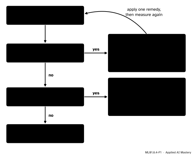
The whole lesson on one page. Two numbers, two questions, two diagnoses, and a list of remedies for each.
“Too high” needs a yardstick: the largest error you are willing to accept. Call it the acceptable error. It might come from what the task needs, from how well a person does the task, or from the noise level if you know it.
Build it up
One example runs through this lesson: the source of lesson 1, with noise \(0.09\). Say an error of \(0.15\) is acceptable.
Step 1. Two sick models. Each is trained on 12 examples. As in lesson 3, the numbers are averages over 2,000 training sets.
| Model | Training error | Validation error |
|---|---|---|
| A: degree 1 | \(0.26\) | \(0.30\) |
| B: degree 9 | \(0.01\) | \(1.00\) |
Step 2. Diagnose. A’s training error, \(0.26\), is above the acceptable \(0.15\). A model that cannot fit even its own examples has high bias. B’s training error is fine and its validation error is not. The trouble is all in the gap: high variance.
Step 3. Treat A. Try four remedies, one at a time, and measure again.
| Remedy for A | Training error | Validation error |
|---|---|---|
| 120 examples | \(0.28\) | \(0.29\) |
| Degree 3 | \(0.06\) | \(0.13\) |
| A sine feature | \(0.07\) | \(0.10\) |
| A penalty | \(0.34\) | \(0.37\) |
Ten times the data moved the validation error by \(0.01\). A richer model fixed it. So did a better feature: the model \(\hat{y} = {w_0 + w_1 \sin(2\pi x)}\), which has two weights like the line but the right shape. (Here we cheat, since we know the truth is a sine. In practice such features come from knowing the problem: a daily cycle, a ratio, a logarithm.) The penalty made A worse.
Step 4. Treat B.
| Remedy for B | Training error | Validation error |
|---|---|---|
| 120 examples | \(0.08\) | \(0.10\) |
| Degree 3 | \(0.06\) | \(0.13\) |
| A penalty | \(0.06\) | \(0.14\) |
All three work. The penalty adds to the loss a price on large weights, which stops the curve from swinging. Module ML01.9 builds it. Here it is only a remedy to try.
Step 5. See why. Split each validation error into its three parts, as lesson 2 did.
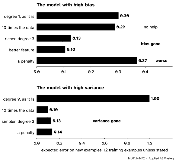
What each remedy does to each part. A remedy works when it shrinks the part that is large. More data shrinks variance, so it rescues B and does nothing for A.
The formal statement
A model can have both problems. The rule then says bias, and that is the right order of work: until the model can fit its own training set, the gap is not worth looking at.
Why each remedy works. Lessons 2 and 3 gave the expected error of a least-squares model with \(p\) parameters and \(n\) training examples. It is exact at the training inputs, and a good estimate elsewhere once \(n\) is several times \(p\):
\[ \E[L_{\text{new}}] = {\underbrace{\sigma^2}_{\text{noise}}} + \text{bias}^2 + {\underbrace{\sigma^2\,\frac{p}{n}}_{\text{variance}}} . \]
Here \(\text{bias}^2\) is the squared bias averaged over inputs, as in lessons 2 and 3. Each remedy moves one piece of this formula.
| Remedy | Bias² | Variance |
|---|---|---|
| More training data | unchanged | falls: \(n\) grows |
| A simpler model | may rise | falls: \(p\) shrinks |
| A richer model | falls | rises: \(p\) grows |
| Better features, same \(p\) | falls | unchanged |
| A stronger penalty | rises a little | falls |
Three things to read off the table.
- More data cannot cure bias. In the formula \(n\) appears only in the variance. For the line, bias² stays near \(0.196\) however many examples arrive.
- A richer model and a simpler model are opposite cures. Each makes the other problem worse, so the diagnosis must come first.
- Nothing in the table touches the noise. Only better measurements, or a new feature that explains part of what looked like noise, can lower \(\sigma^2\).
A penalty does not change \(p\). It shrinks the weights, so the model uses its freedom less. The effect is that of a smaller \(p\): on the example it cut B’s variance from \(0.906\) to \(0.036\) and raised bias² from \(0.000\) to \(0.011\).
Worked example
Diagnose models A and B, then predict what 120 examples would buy before paying for them.
Diagnose. A’s training error is \(0.26\). That is above the acceptable \(0.15\), and \({0.26 - 0.09} = 0.17\) above the noise. Its gap is only \({0.30 - 0.26} = 0.04\). High bias. B’s training error is \(0.01\), which is \(0.08\) below the noise: it has fitted the noise itself. Its gap is \({1.00 - 0.01} = 0.99\). High variance.
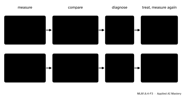
The two diagnoses as a trace, each ending with a remedy that worked and the two errors after it.
Predict. Use the formula as an estimate of the validation error, with \(\sigma^2 = 0.09\) and the average bias² of lesson 2: \(0.196\) for the line and \(0.000\) for degree 9.
Model A, the line: \(p = 2\). The variance term is \({0.09 \cdot 2/12} = 0.015\) with 12 examples and \({0.09 \cdot 2/120} = 0.0015\) with 120. So the estimates are
\[ \begin{aligned} 0.09 + 0.196 + 0.015 &= 0.301, \\ 0.09 + 0.196 + 0.0015 &= 0.2875 . \end{aligned} \]
Ten times the data buys \(0.0135\). The measured values were \(0.301\) and \(0.288\). However large \(n\) grows, A’s error stays above \({0.09 + 0.196} = 0.286\), far over the acceptable \(0.15\).
Model B, degree 9: \(p = 10\). The variance term is \({0.09 \cdot 10/12} = 0.075\) with 12 examples and \({0.09 \cdot 10/120} = 0.0075\) with 120. So the estimates are
\[ \begin{aligned} 0.09 + 0 + 0.075 &= 0.165, \\ 0.09 + 0 + 0.0075 &= 0.0975 . \end{aligned} \]
The measured value at \(n = 120\) was \(0.098\). At \(n = 12\) it was \(1.00\), far above \(0.165\). The formula counts the variance at the training inputs only, and with barely more examples than weights the curves swing far more between and beyond them (lesson 3). There the formula is only a floor. The direction is right, and the prediction for 120 examples is accurate.
How many examples does B need for an error of \(0.10\)? The variance term must be at most \(0.01\): \({0.09 \cdot 10/n} \le 0.01\) gives \(n \ge 90\).
So team A should not buy data. It should change the model. Team B can buy about 90 examples, or switch to degree 3 for nothing.
Code
From scratch: features, two ways of fitting, and a function that measures any combination.
Every row of the tables above, with its diagnosis.
cases = {
    "A: degree 1, 12 examples": (poly(1), 12, 0.0),
    "A + 120 examples": (poly(1), 120, 0.0),
    "A + degree 3": (poly(3), 12, 0.0),
    "A + sine feature": (wave, 12, 0.0),
    "A + penalty 1": (poly(1), 12, 1.0),
    "B: degree 9, 12 examples": (poly(9), 12, 0.0),
    "B + 120 examples": (poly(9), 120, 0.0),
    "B + degree 3": (poly(3), 12, 0.0),
    "B + penalty 0.001": (poly(9), 12, 0.001),
}
results = {name: measure(*case) for name, case in cases.items()}
for name, (train, validation, bias2, variance) in results.items():
    print(f"{name:25s} training {train:.2f}  validation {validation:.2f}  bias^2 {bias2:.3f}  "
          f"variance {variance:.3f}  {diagnose(train, validation, 0.15)}")
A: degree 1, 12 examples training 0.26 validation 0.30 bias^2 0.196 variance 0.015 high bias
A + 120 examples training 0.28 validation 0.29 bias^2 0.196 variance 0.002 high bias
A + degree 3 training 0.06 validation 0.13 bias^2 0.005 variance 0.031 good enough
A + sine feature training 0.07 validation 0.10 bias^2 0.000 variance 0.015 good enough
A + penalty 1 training 0.34 validation 0.37 bias^2 0.269 variance 0.009 high bias
B: degree 9, 12 examples training 0.01 validation 1.00 bias^2 0.000 variance 0.906 high variance
B + 120 examples training 0.08 validation 0.10 bias^2 0.000 variance 0.008 good enough
B + degree 3 training 0.06 validation 0.13 bias^2 0.005 variance 0.031 good enough
B + penalty 0.001 training 0.06 validation 0.14 bias^2 0.011 variance 0.036 good enoughThe library’s penalised least squares is Ridge. Its loss is the sum of the squared errors plus alpha times the sum of squared weights. Ours has the mean of the squared errors in place of the sum, so alpha is n times penalty.
from sklearn.linear_model import Ridge
from sklearn.pipeline import make_pipeline
from sklearn.preprocessing import PolynomialFeatures, StandardScaler

x = inputs(12)
# the first of the 2,000 training sets
y = true_curve(x) + sigma * np.random.default_rng(0).normal(size=(12, 2000))[:, 0]
ours = poly(9)(grid) @ ridge(poly(9)(x), y[:, None], 0.001)[:, 0]
library = make_pipeline(PolynomialFeatures(9, include_bias=False), StandardScaler(),
                        Ridge(alpha=12 * 0.001))
theirs = library.fit(x.reshape(-1, 1), y).predict(grid.reshape(-1, 1))
print(f"largest difference between the two sets of predictions: {np.abs(ours - theirs).max():.1e}")
largest difference between the two sets of predictions: 2.0e-14Explore
Try each remedy yourself in the polynomial fitter of lesson 2. Set degree 9 with 12 points and pile up fits: high variance. Now lower the degree to 3, or switch to 48 points and pile up fits again, and watch the variance in the read-out collapse. Then set degree 1 and try to fix it with more points.
Pitfalls
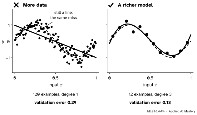
Wrong beside right, for a model with high bias. Ten times the data leaves the line where it was. A richer model fixes it with the twelve examples already there.
“More data always helps.”
It helps variance, and only variance. Model A went from \(0.30\) to \(0.29\) on ten times the data. In machine learning, data is often the most expensive remedy, so check the learning curve before buying it.
“The model is doing badly, so add a penalty.”
A penalty restrains a model. That is the cure for variance and the opposite of the cure for bias: it took model A from \(0.30\) to \(0.37\). If the training error is too high, weaken the restraint.
“Keep trying remedies until the test error looks good.”
Every remedy chosen by looking at a score has been fitted to that score. Diagnose and choose with the validation set. Open the test set once, at the end, for the report (lesson ML01.2.2). Module ML01.9 measures what peeking costs.
Check yourself
Recall
1. Which two measured numbers does the diagnosis need, and what are they compared with?
Show answer
The training error and the validation error, compared with the acceptable error and with each other.
2. The training error is too high. What is the diagnosis? Name two remedies.
Show answer
High bias, or underfitting. Remedies: a richer model, better features, a weaker penalty.
3. The training error is fine and the validation error is far above it. What is the diagnosis? Name three remedies.
Show answer
High variance, or overfitting. Remedies: more data, a simpler model, a stronger penalty.
4. Which part of the error does more training data shrink?
Show answer
The variance. Bias and noise are unchanged.
5. What does a penalty do to bias and to variance?
Show answer
It lowers the variance and raises the bias a little.
Exercises
1. ★ An error of \(0.15\) is acceptable. Diagnose each model from its training and validation error and name one remedy: (a) \(0.50\) and \(0.52\); (b) \(0.05\) and \(0.40\); (c) \(0.11\) and \(0.13\).
Show solution
(a) The training error, \(0.50\), is above \(0.15\): high bias. Use a richer model or better features. (b) The training error is fine and the validation error is not: high variance. Get more data, simplify the model or add a penalty. (c) The validation error is below \(0.15\): good enough. Report the test error.
2. ★★ A least-squares model has \(p = 20\) parameters, no bias, and noise \(\sigma^2 = 0.5\). It is trained on \(n = 50\) examples. (a) Find its expected error. (b) How many examples bring that down to \(0.55\)? (c) A simpler model with \(p = 5\) has bias² \(0.02\). What is its expected error on the same 50 examples?
Show solution
(a) \({0.5 + 0 + {0.5 \cdot 20/50}} = 0.7\).
(b) The variance term must be \(0.05\): \({0.5 \cdot 20/n} = 0.05\) gives \(n = 200\), four times the data.
(c) \({0.5 + 0.02 + {0.5 \cdot 5/50}} = 0.57\). The simpler model gets almost as far as four times the data, for nothing. Its small bias is a good price for the variance it removes.
3. ★★★ Lesson 3 found that the best degree moves from 3 to 5 as the training set grows. Explain it with the formula. Degree 3 has \(p = 4\) and bias² \(0.005\). Degree 5 has \(p = 6\) and bias² \(0.000\). The noise is \(0.09\). From which \(n\) on does degree 5 have the lower expected error?
Show solution
Degree 5 wins when
\[ \begin{aligned} & 0.09 + 0 + 0.09 \cdot \frac{6}{n} \\ & \quad < \; 0.09 + 0.005 + 0.09 \cdot \frac{4}{n} . \end{aligned} \]
Subtract \(0.09\) and \({0.09 \cdot 4/n}\) from both sides: \({0.09 \cdot 2/n} < 0.005\), so \(0.18/n < 0.005\) and \(n > 36\): from 37 examples on. With fewer than 36 the two extra weights cost more in variance than they save in bias, and at exactly 36 the two models tie. With more, the extra weights pay. That matches lesson 3: degree 3 was best at 24 examples and degree 5 at 96.
Summary card
Diagnose first. Then use the remedy that shrinks the part that is large.
Two numbers, two questions, two cures.
- High bias (training error too high): a richer model, better features, a weaker penalty. Not more data.
- High variance (training error fine, validation error far above): more data, a simpler model, a stronger penalty.
- Why. \(\E[L_{\text{new}}] = {\sigma^2 + \text{bias}^2 + \sigma^2 p/n}\): data changes \(n\), model size changes \(p\) and bias², nothing changes \(\sigma^2\).
- One remedy at a time, then measure again. The test set waits until the end.
Sources and next steps
Sources. Each was opened and checked against this lesson on 12 November 2026.
- Andrew Ng, Advice for applying machine learning, CS229 lecture slides, Stanford University. The slide “Diagnostic for bias vs. variance” gives the test: with high variance the training error is much lower than the test error, and with high bias the training error is also high. The slide “Diagnostics tell you what to try next” lists more training examples and a smaller set of features as fixes for high variance, and a larger set of features and new features as fixes for high bias.
- Tengyu Ma and Andrew Ng, CS229 Lecture Notes, Stanford University, Section 8.1. A linear model fitted to a quadratic truth cannot be rescued by more training examples, because the bottleneck is the model family and not the data. Section 8.1.1 notes that the variance term often decreases as the dataset grows and that nothing can be done about the noise term.
- scikit-learn 1.9.1 User Guide, Section 3.5: collect more training data only if the true function is too complex for an estimator with lower variance. Also the API reference for
Ridge, which minimises the sum of squared errors plusalphatimes the sum of squared weights. - Aston Zhang, Zachary Lipton, Mu Li and Alexander Smola, Dive into Deep Learning, Section 3.6. Its summary lists the rules of thumb that more complex models often require more data and that, all else equal, more data almost always leads to better generalisation.
Next. Module ML01.9, Regularization and validation, builds the penalty of this lesson from scratch, shows why it shrinks weights, and makes the choice of its strength a fair one.
This lesson unlocks
ML01.9 Regularization and validation
Your progress is saved in this browser only. No account, no tracking.