Draw the training set again and the fitted curve changes. The expected squared error of a prediction splits into three parts: the squared bias of the average fit, the variance of the fits around it, and the noise. Derive the split step by step and measure each part.
Define the bias, the variance and the noise of a learning method at one input.
Derive, step by step, that the expected squared error is bias squared plus variance plus noise.
Compute bias and variance by hand for a source that has only four possible training sets.
Estimate bias and variance by simulation over many training sets and check their sum against the measured error.
Explain why bias falls and variance rises as a model is made more flexible.
In review. The maths and code on this page are checked by automated tests on every change, but an independent reader has not signed it off yet. Spot a mistake or a confusing step? Tell us.
The question
Lesson 1 fitted polynomials to twelve points. But those twelve points were one draw from the source, and a second draw would have given different curves. If you could repeat the draw two thousand times, what would the cloud of fitted curves tell you about how wrong one fit is likely to be?
From the last lesson
1. Why can the training error not rise when the degree of the polynomial is raised?
Show answer
The larger family contains the smaller one: set the new weight to zero. So its best member fits the training set at least as well.
2. How do underfitting and overfitting show up in the training error and the test error?
Show answer
Underfitting: both are high. Overfitting: the training error is low and the test error is much higher.
Intuition
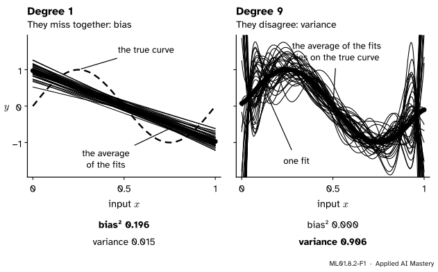
Draw forty training sets from the source of lesson 1, fit each one, and lay the forty fits on top of each other.
ML01.8.2-F1
Forty training sets, forty fits. The lines agree with one another and are wrong in the same place. The degree-9 curves are right on average and disagree with one another.
A cloud of fits can be wrong in two ways.
Its centre can miss the truth. The distance from the average fit to the truth is the bias. The lines have a large one.
It can be wide. The scatter of the fits around their own average is the variance. The degree-9 curves have a large one.
You only ever get one fit from the cloud. It is likely to be far from the truth if the centre is off or the cloud is wide. This lesson makes that exact, and adds a third part that no model can touch: the noise.
Build it up
Step 1. Repeat the experiment. Keep the twelve inputs of lesson 1 and draw fresh noise: that is a new training set. Do it 2,000 times and fit each set.
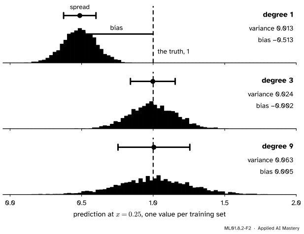
Step 2. Stand at one input. Take \(x_0 = 0.25\), the top of the wave, where the truth is \({\sin(2\pi \cdot 0.25)} = 1\). Each fit makes one prediction there: 2,000 predictions per degree.
ML01.8.2-F2
The 2,000 predictions at \(x_0 = 0.25\). The line’s pile is narrow and in the wrong place. The degree-9 pile is in the right place and wide.
Step 3. Measure the pile. For the line the centre of the pile is \(0.487\), so the bias is \({0.487 - 1} = -0.513\). The spread of the pile, measured as a variance, is \(0.013\). For degree 9 the bias is \(+0.005\) and the variance is \(0.063\).
Step 4. Add the noise. A new target at \(x_0\) is not the truth either. It is the truth plus noise, and the noise has variance \(0.3^2 = 0.09\). Add the three parts and compare with the squared error measured directly on 2,000 new targets.
Degree
1
3
9
Bias²
\(0.263\)
\(0.000\)
\(0.000\)
Variance
\(0.013\)
\(0.024\)
\(0.063\)
Noise
\(0.09\)
\(0.09\)
\(0.09\)
Sum
\(0.366\)
\(0.114\)
\(0.153\)
Measured
\(0.362\)
\(0.114\)
\(0.154\)
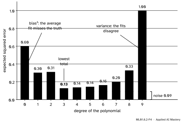
Step 5. Average over all inputs. Do the same at 200 inputs spread over the whole interval and average.
ML01.8.2-F4
The expected error on new examples, in its three parts. Bias falls with the degree, variance rises, the noise never moves. Their sum is the U of lesson 1.
Degree 1 is \({0.196 + 0.015 + 0.09} = 0.301\): nearly all bias. Degree 9 is \({0.000 + 0.906 + 0.09} = 0.996\): nearly all variance. Degree 3 has a little of each, \({0.005 + 0.031 + 0.09} = 0.126\), and the lowest total.
The formal statement
Setting. The source produces \(y = {f(x) + \varepsilon}\), where \(f\) is the true curve and the noise \(\varepsilon\) has mean \(0\) and variance \(\sigma^2\). A training set is drawn and a model is fitted to it. Fix an input \(x_0\) and write
\(f\) for the truth there, \(f(x_0)\);
\(\hat{y}\) for the fitted model’s prediction there, which changes from one training set to the next;
\(m = \E[\hat{y}]\) for the average prediction over all training sets;
\(y_0 = {f + \varepsilon_0}\) for a new target there, whose noise \(\varepsilon_0\) has nothing to do with the training set.
Piece \(a\) is the new example’s noise, \(\varepsilon_0\). Piece \(b\) is minus the bias, a fixed number. Piece \(c\) says how far this fit is from the average fit.
In the first two results \(b\) is a fixed number, so it comes out of the average. The third uses independence: the new noise \(\varepsilon_0\) knows nothing of the training set, and the average of a product of independent quantities is the product of their averages (lesson ML01.2.3).
Step 5. Add. The six averages sum to \({\sigma^2 + \text{bias}^2 + \text{variance}}\).
Three things follow.
The noise is a floor. Bias² and variance are never negative, so no model has an expected error below \(\sigma^2\).
Averages of the three parts add too. Averaging the result over many inputs \(x_0\) gives the expected test error as average bias² plus average variance plus noise.
Flexibility trades one part for the other. A richer family can bring its average fit closer to the truth, so bias falls. It also has more freedom to follow each training set’s noise, so variance rises.
Go deeper: exact bias and variance for least squares, without simulation
Lesson 1 showed that a least-squares prediction is a weighted sum of the training targets, \(\hat{y} = \sum_i s_i\,y_i\), with weights \(s_i\) that depend only on the inputs. Put \(y_i = {f(x_i) + \varepsilon_i}\):
The first sum is a fixed number and the second has mean \(0\), so \(m = \sum_i s_i f(x_i)\). The second sum is \({\hat{y} - m}\). Its terms are independent, and scaling a quantity by \(s_i\) scales its variance by \(s_i^2\) (Facts A and B of lesson ML01.2.3), so
\[
\text{variance} = \sigma^2 \sum_i s_i^2 .
\]
At \(x_0 = 0.25\) these formulas give a bias of \(-0.514\), \(-0.007\) and \(0.000\) for degrees 1, 3 and 9, and a variance of \(0.0132\), \(0.0242\) and \(0.0617\). The simulated values lie within one and a half standard errors (lesson ML01.2.3) of these. At \(x_0 = 0\) the degree-11 weights of lesson 1 have \(\sum_i s_i^2 \approx 84{,}500\), so the variance there is about \(7{,}600\).
Frontier note: double descent: past the peak, error can fall again
The U-shaped curve is not the whole story. Belkin, Hsu, Ma and Mandal (2019) describe a double descent curve: test error rises as a model approaches the size at which it can fit the training set exactly, and then, for still larger models, falls again. The peak sits where the number of parameters is about the number of examples, which is exactly where the degree-11 polynomial sits on twelve points. Large neural networks are often trained beyond that peak. The decomposition of this lesson still holds there. The rule of thumb that a model must get worse once it can fit its training set exactly does not.
Worked example
Count the bias and variance of two models by hand.
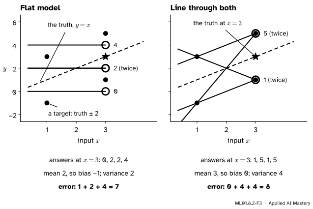
A tiny source: the truth is \(f(x) = x\), and the noise is a coin flip, \(+2\) or \(-2\), so \(\sigma^2 = 4\). A training set has two examples, one at \(x = 1\) and one at \(x = 3\). The target at \(x = 1\) is \(-1\) or \(3\), and the target at \(x = 3\) is \(1\) or \(5\): four equally likely training sets.
Two models predict at \(x_0 = 3\), where the truth is \(3\).
The flat model answers with the mean of the two targets.
The line passes through both points, so at \(x = 3\) it answers with the target there.
Training targets
Flat model
Line
\(-1\) and \(1\)
\(0\)
\(1\)
\(-1\) and \(5\)
\(2\)
\(5\)
\(3\) and \(1\)
\(2\)
\(1\)
\(3\) and \(5\)
\(4\)
\(5\)
Flat model. The average answer is \(m = {(0 + 2 + 2 + 4)/4} = 2\), so the bias is \({2 - 3} = -1\). The distances from \(m\) are \(-2, 0, 0, 2\), so the variance is \({(4 + 0 + 0 + 4)/4} = 2\). The expected squared error is \({(-1)^2 + 2 + 4} = 7\).
Line. The average answer is \({(1 + 5 + 1 + 5)/4} = 3\), so the bias is \(0\). The distances from \(m\) are \(-2, 2, -2, 2\), so the variance is \(16/4 = 4\). The expected squared error is \({0 + 4 + 4} = 8\).
ML01.8.2-F3
All four training sets, both models. The flat model’s answers are centred on 2, one below the truth, and close together. The line’s answers are centred on the truth and far apart.
Check by counting. For the flat model, pair each of its four answers with each of the two possible new targets, \(1\) and \(5\). The eight squared errors are \(1, 1, 1, 9\) against the target \(1\) and \(25, 9, 9, 1\) against the target \(5\). Their mean is \(56/8 = 7\), as the formula says.
The model that is right on average loses to the model that is wrong on average, \(8\) against \(7\). The line pays more in variance than the flat model pays in bias.
Code
The worked example first, in plain Python: list the four training sets and count.
from itertools import producttruth =lambda x: x # the coin-flip source: y = x, plus or minus 2flat =lambda y1, y3, x: (y1 + y3) /2# the mean of the two targetsline =lambda y1, y3, x: y1 + (y3 - y1) * (x -1) /2# the line through (1, y1) and (3, y3)x0 =3for name, model in [("flat", flat), ("line", line)]:# the model's answer at x0 for each of the four training sets answers = [model(1+ e1, 3+ e3, x0) for e1, e3 in product([-2, 2], repeat=2)] mean =sum(answers) /4 bias = mean - truth(x0) variance =sum((a - mean) **2for a in answers) /4# the squared error in all eight cases: four training sets, two new targets direct =sum((truth(x0) + e0 - a) **2for a in answers for e0 in [-2, 2]) /8print(f"{name}: answers {answers} bias {bias:+.0f} variance {variance:.0f} "f"bias^2 + variance + noise = {bias **2+ variance +4:.0f} "f"counted directly: {direct:.0f}")
The library fits one training set at a time. On the first 200 sets a scikit-learn pipeline matches the code above.
from sklearn.linear_model import LinearRegressionfrom sklearn.pipeline import make_pipelinefrom sklearn.preprocessing import PolynomialFeaturesmodel = make_pipeline(PolynomialFeatures(3), LinearRegression())library = np.array([model.fit(x.reshape(-1, 1), Y[:, k]).predict([[x0]])[0] for k inrange(200)])W, *_ = np.linalg.lstsq(powers(x, 3), Y[:, :200], rcond=None)scratch = powers(np.array([x0]), 3)[0] @ Wprint(f"degree 3, 200 training sets: variance {library.var():.4f} with scikit-learn, "f"{scratch.var():.4f} from scratch")
degree 3, 200 training sets: variance 0.0239 with scikit-learn, 0.0239 from scratch
Explore
ML01.8-X1
Polynomial fitter
It opens on the twelve points of lesson 1. Choose a degree, then press New training set a few times and watch the fitted curve jump. Press Add 50 to pile up fits: the thick curve is their average, and the read-out splits the error into bias², variance and noise. Then try 48 training points and see what happens to the variance.
Pitfalls
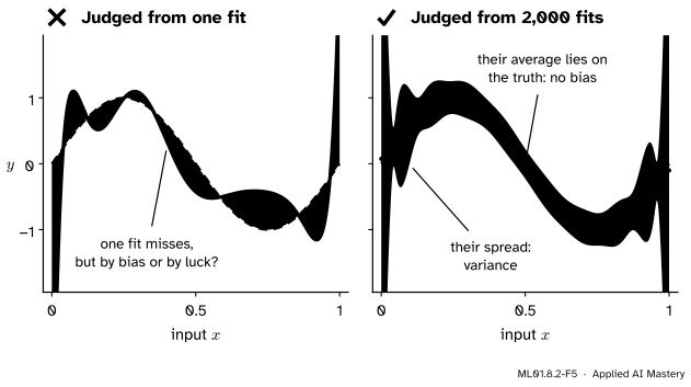
ML01.8.2-F5
Wrong beside right. One fit cannot show bias. The average of many fits can, and here it shows none.
“This fitted curve misses the truth, so the model is biased.”
A single fit misses for two reasons mixed together. Bias is what is left after averaging over training sets. The degree-9 polynomial has almost none, and every one of its misses is variance.
“Variance is the noise in the data.”
Noise is how far a target lies from the truth. Variance is how far a fit moves when the training set is redrawn. Noise causes variance, but they are different numbers: here the noise is \(0.09\) for every model, while the variance runs from \(0.007\) to \(0.906\).
“Less bias always costs more variance.”
That is what turning the flexibility dial does. Other moves escape the trade: more training data lowers variance without touching bias, and a better feature can lower bias without adding variance. Lesson 4 uses both. This is why machine learning cares so much about data and features, and not only about model size.
Check yourself
Recall
1. Define the bias of a learning method at an input \(x_0\).
Show answer
The average prediction at \(x_0\) over all training sets, minus the truth there: \({m - f}\).
2. Define its variance at \(x_0\).
Show answer
The average squared distance of the prediction from the average prediction, \({\E[(\hat{y} - m)^2]}\): how much the fit moves when the training set is redrawn.
3. State the decomposition of the expected squared error.
Show answer
\({\E[(y_0 - \hat{y})^2]} = {\text{bias}^2 + \text{variance} + \text{noise}}\), where the noise is \(\sigma^2\).
4. Why does the cross term between the new example’s noise and the fit’s error vanish?
Show answer
The new noise is independent of the training set and has mean \(0\), so the average of the product is the product of the averages, which is \(0\).
5. As the degree of the polynomial rises, what happens to bias², variance and noise?
Show answer
Bias² falls, variance rises, the noise stays the same. Their sum falls and then rises.
Exercises
1.★ Over five training sets, a model’s predictions at one input are \(2, 4, 3, 5\) and \(6\). The truth there is \(5\) and the noise variance is \(1\). Find the bias, the variance and the expected squared error.
Show solution
The mean prediction is \({(2 + 4 + 3 + 5 + 6)/5} = 4\), so the bias is \({4 - 5} = -1\). The distances from the mean are \(-2, 0, -1, 1, 2\), so the variance is \({(4 + 0 + 1 + 1 + 4)/5} = 2\). The expected squared error is \({(-1)^2 + 2 + 1} = 4\).
2.★★ In the coin-flip source of the worked example, both models now predict at \(x_0 = 4\), where the truth is \(4\). The line through \((1, y_1)\) and \((3, y_3)\) predicts \({y_1 + {1.5\,(y_3 - y_1)}}\) there. Find the bias, variance and expected squared error of each model.
Show solution
Flat model. Its answers do not depend on \(x_0\): they are \(0, 2, 2, 4\) again, with mean \(2\) and variance \(2\). The bias is \({2 - 4} = -2\), and the error is \({4 + 2 + 4} = 10\).
Line. For the targets \((-1, 1)\), \((-1, 5)\), \((3, 1)\) and \((3, 5)\) it predicts \({-1 + 3} = 2\), \({-1 + 9} = 8\), \({3 - 3} = 0\) and \({3 + 3} = 6\). The mean is \(16/4 = 4\), so the bias is \(0\). The distances from the mean are \(-2, 4, -4, 2\), so the variance is \({(4 + 16 + 16 + 4)/4} = 10\). The error is \({0 + 10 + 4} = 14\).
Beyond the training inputs the line’s variance has grown from \(4\) to \(10\): small changes in the two targets swing the far end of the line.
3.★★★ Change the truth of the coin-flip source to \(f(x) = s\,x\) for a slope \(s\), keeping the noise. For which slopes does the flat model have a lower expected squared error than the line at \(x_0 = 3\)?
Show solution
Flat model. The targets are \({s \pm 2}\) and \({3s \pm 2}\), so its answers are \({2s - 2}\), \(2s\), \(2s\) and \({2s + 2}\). Their mean is \(2s\) and their variance is still \({(4 + 0 + 0 + 4)/4} = 2\). The truth at \(x_0 = 3\) is \(3s\), so the bias is \({2s - 3s} = -s\) and the error is \({s^2 + 2 + 4}\).
Line. It answers with the target at \(x = 3\), which is \({3s \pm 2}\): bias \(0\), variance \(4\), error \({0 + 4 + 4} = 8\).
The flat model wins when \({s^2 + 6} < 8\), that is when \(s^2 < 2\), or \(-1.41 < s < 1.41\). A biased model beats an unbiased one whenever the pattern it ignores is small beside the noise.
Sources. Each was opened and checked against this lesson on 12 November 2026.
Tengyu Ma and Andrew Ng, CS229 Lecture Notes, Stanford University. Section 8.1 introduces bias and variance with polynomial fits of several training sets. Section 8.1.1 derives the decomposition for a fixed test input (equations 8.2 to 8.7): unavoidable noise \(\sigma^2\), plus the squared distance from the truth to the average model, plus the variance of the fitted model. Section 8.2 describes double descent, with a peak where the model can just fit all the training data.
Gareth James, Daniela Witten, Trevor Hastie, Robert Tibshirani and Jonathan Taylor, An Introduction to Statistical Learning with Applications in Python, Springer, 2023, Section 2.2.2. Equation 2.7 states that the expected test error at \(x_0\) is the variance of the fit plus its squared bias plus the variance of the error term, which is called the irreducible error.
Ian Goodfellow, Yoshua Bengio and Aaron Courville, Deep Learning, MIT Press, 2016, Section 5.4.4. Equations 5.53 and 5.54 write the mean squared error of an estimator as bias squared plus variance, and Figure 5.6 shows bias falling and variance rising with capacity.
Mikhail Belkin, Daniel Hsu, Siyuan Ma and Soumik Mandal, Reconciling modern machine learning practice and the bias-variance trade-off, published in 2019. Its double-descent curve extends the U-shaped curve beyond the point where a model fits its training data exactly, and peaks at that point, which for their random-feature models is where parameters equal examples.
Next.ML01.8.3 Learning curves shows how to tell bias from variance when you cannot redraw the training set: by watching the two errors as the training set grows.