Differentiate the sigmoid, then the log loss, and the gradient collapses to prediction minus label, times the feature. Train logistic regression from scratch, match scikit-learn’s LogisticRegression, and see what its default regularisation changes.
Derive the derivative of the sigmoid and show that it equals p times one minus p.
Derive the gradient of the log loss with the chain rule, and explain why it has the same form as the gradient for a line.
Carry out one gradient descent update of logistic regression by hand.
Train logistic regression from scratch in NumPy and reproduce scikit-learn’s fit, with and without its default regularisation.
Explain why the weights grow without limit on data that a single cut separates perfectly.
In review. The maths and code on this page are checked by automated tests on every change, but an independent reader has not signed it off yet. Spot a mistake or a confusing step? Tell us.
The question
The log loss scores any curve, and the best curve has the lowest score. For a straight line there was a formula for the best parameters. Here there is none, so we must walk downhill, and for that we need the slope of a loss made of logarithms of sigmoids. It looks like a long calculation. It ends in almost the same two lines as the slope for a straight line. Why?
Training is the loop of module ML01.5: measure the two slopes of the loss where you stand, step against them, repeat. Only the model and the loss have changed. The model is now \({p = {\sigma(wx + b)}}\) and the loss is the log loss \({L(w, b)}\) of the six students.
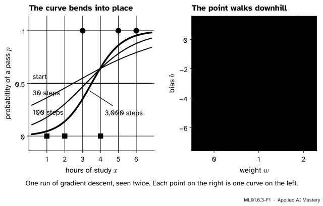
ML01.6.3-F1
One run of gradient descent, seen twice. Left: the model starts as the flat coin-flip line and bends into an S. Right: the same run as a path on the map of the log loss, from the origin down a long valley to the lowest point.
Here is the result we are heading for, in words. Call \({p_i - y_i}\) the miss of student \(i\): the predicted probability minus the label. It is positive when the model said too much “pass” and negative when it said too little. Then
the slope of the loss along \(b\) is the average miss, and
the slope along \(w\) is the average of miss times hours.
Each student pulls the curve towards their own mark, with a force equal to the miss.
Build it up
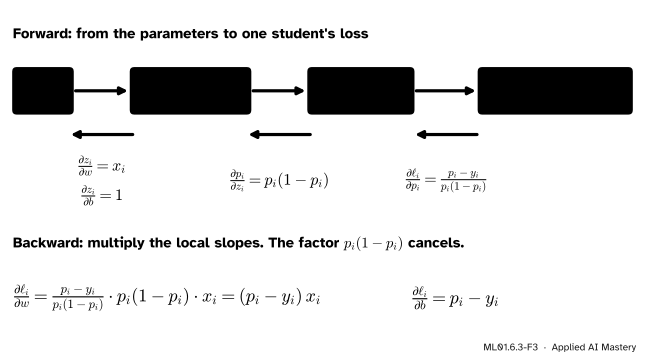
Step 1. The loss is a chain. From the parameters to one student’s loss there are three links: the score \({z_i = w x_i + b}\), the probability \({p_i = \sigma(z_i)}\), and the loss \(\ell_i = {-[\,y_i \ln p_i + (1 - y_i)\ln(1 - p_i)\,]}\). The log loss \(L\) is the mean of the \(\ell_i\). The chain rule says: to get the slope of the end with respect to the start, multiply the slopes of the links.
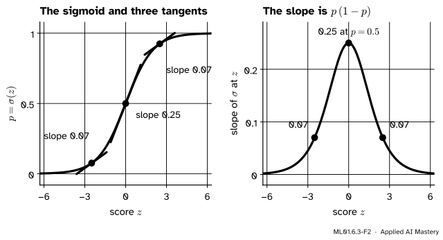
Step 2. The one new link is the sigmoid. Its slope is largest in the middle and fades to nothing at both ends, where the curve is flat.
ML01.6.3-F2
Left: the sigmoid with three tangent lines. Right: the slope of the sigmoid at every score. It peaks at \(\tfrac14\), where \({p = \tfrac12}\), and it equals \({p\,(1 - p)}\) everywhere.
Step 3. Multiply the links, and something cancels. The slope of the loss with respect to \(p\) turns out to carry \({p(1 - p)}\) in its denominator. The slope of the sigmoid is \({p(1 - p)}\). Their product is just the miss.
ML01.6.3-F3
The chain for one student. Going backward, each link contributes one local slope. Two of them cancel, and the product is the miss times whatever multiplies the parameter in the score.
Step 4. Compare with the line. For a line with the mean squared error, ML01.5 found \(\pd{L}{w} = {\frac{2}{n}\sum_i (\hat{y}_i - y_i)\,x_i}\). The new slope has the same shape: prediction minus target, times input, averaged. Only two things differ. The prediction is now \({\sigma(w x_i + b)}\), and the factor \(2\) is gone.
Step 5. Step against the gradient. With a learning rate \(\eta\),
\[
w \leftarrow w - \eta\,\pd{L}{w}, \qquad b \leftarrow b - \eta\,\pd{L}{b} ,
\]
both slopes measured at the current point before either parameter moves.
The formal statement
NoteResult: the gradient of the log loss
For the log loss \({L(w, b)}\) of lesson 2, with \({p_i = {\sigma(w x_i + b)}}\),
So \(\frac{dp}{dz} = {p\,(1 - p)}\). At \({z = 0}\) it is \({\tfrac12 \cdot \tfrac12} = \tfrac14\), its largest value.
Part B: the loss of one student with respect to \(p\). Drop the index for a moment: \(\ell = {-[\,y \ln p + (1 - y)\ln(1 - p)\,]}\). The slope of \(\ln p\) is \(\tfrac1p\), and the slope of \({\ln(1 - p)}\) is \({-\tfrac{1}{1 - p}}\).
Part D: the mean.\(L\) is the mean of the \(\ell_i\), and the slope of a mean is the mean of the slopes. That gives the boxed result.
What the gradient says at the bottom. At the lowest point both slopes are zero. From \({\pd{L}{b} = 0}\) we get \({\sum_i p_i = \sum_i y_i}\): the predicted probabilities add up to the number of passes that were seen. But unlike the line, these two equations cannot be solved by algebra, because \(w\) and \(b\) sit inside an exponential inside each \(p_i\). That is why logistic regression is trained by iteration.
More than one feature. With features \({x_{i1}, \dots, x_{id}}\) the score is \(z_i = w_1 x_{i1} + \dots + w_d x_{id} + b\). Only the last link changes: \({\pd{z_i}{w_j} = x_{ij}}\). So \(\pd{L}{w_j} = {\frac{1}{n}\sum_i (p_i - y_i)\,x_{ij}}\). Stack the examples as the rows of a matrix \(\mat{X}\) and the whole gradient is one line, \(\nabla_{\vect{w}} L = {\frac{1}{n}\,\mat{X}\T(\vect{p} - \vect{y})}\).
Go deeper: why there is one valley, and how large the learning rate may be
Differentiate \({\frac{d\ell}{dz} = p - y}\) once more: \(\frac{d^2\ell}{dz^2} = \frac{dp}{dz} = {p(1 - p)}\), which is positive. So each student’s loss curves upward as a function of the score, and the score is a straight-line function of \(w\) and \(b\). A mean of such functions is convex: it has no separate dips and no flat shelves, only one valley.
The same number bounds the curvature. Since \({{p(1 - p)} \le \tfrac14}\), the loss never curves more sharply than a quadratic bowl whose second derivatives are \(\tfrac14\) of the averages of \(x_i^2\), \(x_i\) and \(1\). For the six students the larger eigenvalue of that bowl is \(4.00\). Let the bowl touch the loss where you stand, with the same slope. The loss bends less, so it stays below the bowl, and one step of gradient descent is the same step on both. By the rule of ML01.5.3, any learning rate below \({2 / 4.00 = 0.50}\) lowers the bowl, so it lowers the loss too. This lesson uses \({\eta = 0.3}\).
Frontier note: the first line of every backward pass
A deep network for classification ends in a sigmoid, or in its many-class version the softmax, followed by the log loss. Backpropagation starts at that end, and its first result is the one derived here: the slope of the loss with respect to the final score is prediction minus label.
Worked example
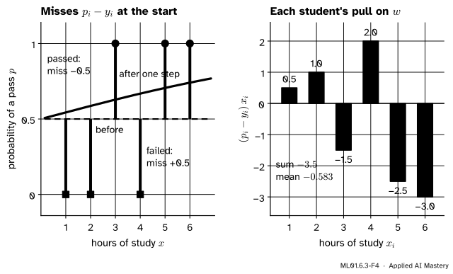
One update by hand, from \({w = 0}\), \({b = 0}\), with learning rate \({\eta = 0.3}\).
At the start every score is \(0\), so every prediction is \({\sigma(0) = 0.5}\).
The first update. Left: every miss is half a unit, up or down. Right: multiplied by the hours, the misses of the hard-working students weigh most, and the total is negative, so \(w\) goes up.
Why did only \(w\) move? Three misses of \(+0.5\) and three of \(-0.5\) cancel, so the average miss is zero: a flat line at \(0.5\) already predicts the right number of passes. But the passes sit at longer hours than the fails, so the misses weighted by hours do not cancel. The curve must tilt.
Did the loss fall? Before the step it was \({\ln 2 = 0.693}\). The new curve \({p = {\sigma(0.175\,x)}}\) gives the six probabilities
The second step. Now every prediction is above \(0.5\), so the average miss is positive, \({\pd{L}{b} = 0.146}\), and the bias is pulled down. With \({\pd{L}{w} = 0.041}\) the new point is \({(w, b)} = {(0.163, -0.044)}\) and the loss is \(0.641\). From here the two parameters travel together down the valley of the map: \(w\) up, \(b\) down.
The end of the run. After 3,000 steps the parameters have stopped changing at \({w = 1.214}\), \({b = -4.249}\), with \({L = 0.413}\). The curve crosses one half at \({-b/w = 3.50}\) hours.
Code
From scratch. The gradient function is the boxed result, line for line.
import numpy as nphours = np.array([1.0, 2.0, 3.0, 4.0, 5.0, 6.0])passed = np.array([0.0, 0.0, 1.0, 0.0, 1.0, 1.0])def sigmoid(z):return1.0/ (1.0+ np.exp(-z))def log_loss(w, b, x=hours, y=passed): z = w * x + breturn np.mean(np.logaddexp(0.0, z) - y * z) # the stable form: ln(1 + e^z) - y zdef gradient(w, b, x=hours, y=passed): miss = sigmoid(w * x + b) - y # p - y, one entry per studentreturn np.mean(miss * x), np.mean(miss)def train(w, b, lr, steps, x=hours, y=passed, penalty=0.0):for _ inrange(steps): dw, db = gradient(w, b, x, y) # both slopes at the current point ... w, b = w - lr * (dw +2* penalty * w), b - lr * db # ... then both parameters movereturn w, bprint("gradient at (0, 0):", np.round(gradient(0.0, 0.0), 3))for steps in [1, 2, 100, 1000, 3000]: w, b = train(0.0, 0.0, lr=0.3, steps=steps)print(f"after {steps:>4} steps: w = {w:.4f}, b = {b:8.4f}, L = {log_loss(w, b):.4f}")
gradient at (0, 0): [-0.583  0.   ]
after    1 steps: w = 0.1750, b =   0.0000, L = 0.6474
after    2 steps: w = 0.1626, b =  -0.0437, L = 0.6414
after  100 steps: w = 0.7010, b =  -2.2276, L = 0.4525
after 1000 steps: w = 1.2051, b =  -4.2143, L = 0.4130
after 3000 steps: w = 1.2140, b =  -4.2491, L = 0.4130
The first two rows match the worked example. The penalty argument is not used yet. Before trusting the gradient, check it against finite differences, as in ML01.5.2.
def numerical_gradient(w, b, h=1e-5): dw = (log_loss(w + h, b) - log_loss(w - h, b)) / (2* h) db = (log_loss(w, b + h) - log_loss(w, b - h)) / (2* h)return dw, dbrng = np.random.default_rng(0)worst =0.0for _ inrange(100): w, b = rng.uniform(-3, 3), rng.uniform(-8, 8) worst =max(worst, np.abs(np.subtract(gradient(w, b), numerical_gradient(w, b))).max())print(f"largest gap between the formula and the measurement at 100 points: {worst:.1e}")
largest gap between the formula and the measurement at 100 points: 1.6e-10
Now the library. scikit-learn’s LogisticRegression does not minimise the log loss alone. By default it adds a penalty on the size of the weight, \({\frac{1}{2nC}\,w^2}\) with \({C = 1}\), which ML01.9 studies under the name regularisation. Setting C=np.inf switches the penalty off.
from sklearn.linear_model import LogisticRegressionX = hours.reshape(-1, 1) # scikit-learn wants one column per featuredefault = LogisticRegression().fit(X, passed)plain = LogisticRegression(C=np.inf).fit(X, passed)w_gd, b_gd = train(0.0, 0.0, lr=0.3, steps=3000)w_pen, b_pen = train(0.0, 0.0, lr=0.3, steps=3000, penalty=1/ (2*6*1.0)) # 1 / (2 n C)print(f"scikit-learn, default (C = 1): w = {default.coef_[0, 0]:.3f}, b = {default.intercept_[0]:.3f}")print(f"from scratch, with the penalty: w = {w_pen:.3f}, b = {b_pen:.3f}")print(f"scikit-learn, C = np.inf: w = {plain.coef_[0, 0]:.3f}, b = {plain.intercept_[0]:.3f}")print(f"from scratch, no penalty: w = {w_gd:.3f}, b = {b_gd:.3f}")
scikit-learn, default (C = 1):  w = 0.767, b = -2.685
from scratch, with the penalty: w = 0.767, b = -2.685
scikit-learn, C = np.inf:       w = 1.214, b = -4.249
from scratch, no penalty:       w = 1.214, b = -4.249
The default model has a smaller weight, \(0.767\) instead of \(1.214\): a gentler curve with the same midpoint. Neither is wrong. They minimise different losses, and you must know which one you asked for.
Two short experiments finish the picture. First, speed: centre the hours and the long valley becomes a round bowl, as ML01.5.3 promised, so 300 steps do what took 3,000.
centred = hours - hours.mean() # hours above or below 3.5w_c, b_c = train(0.0, 0.0, lr=0.3, steps=300, x=centred)print(f"centred, 300 steps: w = {w_c:.4f}, b = {b_c - w_c * hours.mean():.4f} (converted back to raw hours)")separable = np.array([0.0, 0.0, 0.0, 1.0, 1.0, 1.0]) # swap two labels: now 3.5 hours splits them perfectlyfor steps in [100, 10_000, 100_000]: w, b = train(0.0, 0.0, lr=0.3, steps=steps, y=separable)print(f"separable, {steps:>7,} steps: w = {w:6.2f}, L = {log_loss(w, b, y=separable):.4f}")w, b = train(0.0, 0.0, lr=0.3, steps=10_000, y=separable, penalty=1/12)print(f"separable, with the penalty: w = {w:.2f}")
centred, 300 steps: w = 1.2140, b = -4.2491 (converted back to raw hours)
separable,     100 steps: w =   0.97, L = 0.2710
separable,  10,000 steps: w =   5.99, L = 0.0165
separable, 100,000 steps: w =  10.48, L = 0.0018
separable, with the penalty: w = 1.12
Second, the surprise in the last four lines. With two labels swapped, every student who failed studied less than every one who passed, and the weight never settles: a steeper curve always fits a little better. The pitfalls section returns to this.
Explore
ML01.6-X1
Sigmoid and boundary explorer
Move the weight and bias sliders and watch the curve, the purple gap at each student and the bar chart of log losses. Switch to Two features for the ten students of lesson 4.
Three things to try. Press Step once after Reset and compare the read-out with the worked example: \({w = 0.175}\), \({b = 0}\), \({L = 0.647}\). Press Train and watch the step counter race ahead while the curve barely moves: that is the long valley. Last, set \({w = 6}\) and \({b = -21}\), almost a step at 3.5 hours. Two bars dwarf the rest: the students with three and four hours, who are why the best curve stays gentle.
Pitfalls
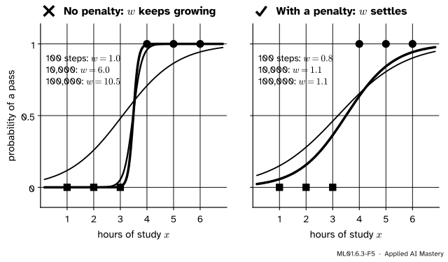
ML01.6.3-F5
Wrong beside right, on six students that a cut at 3.5 hours separates perfectly. Left: plain gradient descent on the log loss never stops steepening the curve. Right: with scikit-learn’s default penalty the weight settles at \(1.12\).
“Train long enough and the weights always settle.”
Not when a cut separates the two classes perfectly. Then every steeper curve has a lower loss, the loss can approach \(0\) but never reach it, and the weight grows without limit: \(0.97\), \(5.99\), \(10.48\) after a hundred, ten thousand and a hundred thousand steps. The model ends up certain about students it has no grounds to be certain about. A penalty on the weights, or stopping early, gives a finite answer.
“scikit-learn gives different numbers, so my code is wrong.”
Check the defaults first. LogisticRegression() applies an L2 penalty with \({C = 1}\), so it returned \({w = 0.767}\) where plain gradient descent found \(1.214\). With C=np.inf the two agree. On a large dataset the default penalty hardly matters. On six students it cuts the weight by over a third.
“The update adds \({(p - y)\,x}\) to the weight.”
The gradient is \({(p - y)\,x}\), and gradient descent subtracts the gradient. So the weight moves by \({+\eta\,(y - p)\,x}\). Many books write the update in that second form. Mixing the two conventions flips the sign, and the loss then climbs from the first step.
Check yourself
Recall
1. What is the derivative of the sigmoid, written with \({p = \sigma(z)}\)? Where is it largest?
Show answer
\(\frac{dp}{dz} = {p\,(1 - p)}\). It is largest at \({z = 0}\), where \({p = \tfrac12}\) and the slope is \(\tfrac14\).
2. Write the two partial derivatives of the log loss of logistic regression.
3. How do they differ from the gradient of the mean squared error of a line?
Show answer
They have the same form: prediction minus target, times the input, averaged. The prediction is now \({\sigma(w x_i + b)}\) instead of \({w x_i + b}\), and there is no factor \(2\).
4. At \({w = 0}\), \({b = 0}\) the slope along \(b\) was zero for the six students. Why?
Show answer
Every prediction is \(0.5\), so three misses are \(+0.5\) and three are \(-0.5\). Their average is zero.
5. What does scikit-learn’s LogisticRegression do by default that plain gradient descent on the log loss does not?
Show answer
It adds an L2 penalty on the weights, with strength set by \({C = 1}\). C=np.inf removes it.
Exercises
1.★ Compute the gradient at \({{(w, b)} = {(1, -3.5)}}\) by hand, using the six probabilities of lesson 1, from \(0.076\) for one hour to \(0.924\) for six. Which way should \(w\) move?
with sum \(-0.304\), so \(\pd{L}{w} = -0.304 / 6 = -0.051\). The slope along \(w\) is negative, so \(w\) should increase. That agrees with the trained value \(1.214\), which is above \(1\).
2.★★ Replace the log loss by the squared error of the probabilities, \(L = {\frac{1}{n}\sum_i (p_i - y_i)^2}\). Derive \(\pd{L}{w}\). Then, for one student who passed and whose score is \({z = -5}\), compare the slope with respect to \(z\) under the two losses.
Show solution
For one student \({\ell = {(p - y)^2}}\), so \(\frac{d\ell}{dp} = {2\,(p - y)}\). The other links are unchanged: \(\frac{dp}{dz} = {p\,(1 - p)}\) and \({\pd{z}{w} = x}\). Hence \(\frac{d\ell}{dz} = {2\,(p - y)\,p\,(1 - p)}\) and
Nothing cancels the factor \({p\,(1 - p)}\) this time. At \({z = -5}\), \({p = 0.0067}\) and \({y = 1}\). The log-loss slope is \({p - y = -0.993}\). The squared-error slope is
about 75 times smaller. This is the flat shelf of lesson 2, now with its cause: the sigmoid’s own slope, which is tiny wherever the model is confident.
3.★★★ Take the separable labels \({y = {(0, 0, 0, 1, 1, 1)}}\) for \({x = 1, \dots, 6}\) and the family of curves \({w = s}\), \({b = -3.5\,s}\) with \({s > 0}\). Write the log loss as a function of \(s\), and show that it decreases for ever, so that no finite \(s\) is best.
Show solution
The score of student \(i\) is \({s\,(x_i - 3.5)}\): \({-2.5s},\ {-1.5s},\ {-0.5s}\) for the three fails and \({0.5s,\ 1.5s,\ 2.5s}\) for the three passes. A fail with score \(z\) costs \({\ln(1 + e^{z})}\) and a pass costs \({\ln(1 + e^{-z})}\) (lesson 2). Every student is on the correct side, so all six costs have the form \({\ln(1 + e^{-ks})}\) with \({k = 0.5,\ 1.5,\ 2.5}\), each value twice:
As \(s\) grows, each \(e^{-ks}\) shrinks, so each logarithm shrinks, and \(L(s)\) is strictly decreasing. It tends to \({\ln 1 = 0}\) and never reaches it, because \(e^{-ks}\) is never \(0\). So for every \(s\) there is a better one, and the loss has no lowest point. On the original labels this cannot happen: there the students with three and four hours are on the wrong side, their costs grow with \(s\), and the two effects balance at \({s = 1.214}\).
Summary card
The slope of the log loss is the miss, prediction minus label, times the input.
ML01.6.3-F1
The curve bends as the point descends.
Sigmoid slope.\(\frac{dp}{dz} = {p\,(1 - p)}\), at most \(\tfrac14\).
Watch for. Separable data: without a penalty the weights never stop growing.
Sources and next steps
Sources. Each was opened and checked against this lesson on 12 November 2026.
Tengyu Ma and Andrew Ng, CS229 Lecture Notes, Stanford University, Section 2.1. Derives \({g'(z) = {g(z)(1 - g(z))}}\) for the sigmoid and the slope of the log-likelihood of one example, \({(y - h_\theta(x))\,x_j}\) (equation 2.2), and remarks that the update looks identical to the one for least squares. They maximise the log-likelihood, so their sign is the opposite of ours.
Daniel Jurafsky and James H. Martin, Speech and Language Processing, 3rd edition draft of 19 August 2026, Chapter 4. Section 4.6 states the gradient as \({(\hat{y} - y)\,x_j}\) for a weight (equation 4.26) and \({\hat{y} - y}\) for the bias (4.28). Section 4.15 derives it, using the derivative of the sigmoid (4.58), and Section 4.8 finds the same form with the softmax (4.41).
scikit-learn 1.9 documentation, LogisticRegression: “regularization is applied by default”, \(C\) defaults to \(1.0\), and C=np.inf gives unpenalised logistic regression. The User Guide, Section 1.1.11, gives the objective as the mean log loss plus \({r(w)/(S\,C)}\) with \({r(w) = \tfrac12 w\T w}\) and \(S\) the total sample weight, \(n\) when every weight is \(1\): the penalty \(\frac{1}{2nC}w^2\) of the code.