Derive the two slopes of the mean squared error with the chain rule, pack them into the gradient, and step against it. One update is worked by hand, then gradient descent is built in NumPy and checked against the exact least-squares answer.
Derive both partial derivatives of the mean squared error of a line with the chain rule.
Explain why the gradient points uphill and why the update rule subtracts it.
Carry out one gradient descent update by hand, from the residuals to the new parameters.
Implement gradient descent in NumPy and check its gradient with finite differences.
In review. The maths and code on this page are checked by automated tests on every change, but an independent reader has not signed it off yet. Spot a mistake or a confusing step? Tell us.
The question
On a curve there are two ways to move, left or right, and the sign of one slope chooses between them. On a landscape you can step in any direction of the compass. Which of them is downhill, and how far should one step go? The answer is a two-line rule, and the same rule, with refinements, trains nearly every neural network.
From the last lesson
1. When we call the loss a function, what is its input and what stays fixed?
Show answer
The input is the parameters, the pair \((w, b)\). The examples stay fixed.
2. The slope of the loss at your current \(w\) is negative. Which way should \(w\) move?
Show answer
Up. The loss falls as \(w\) increases, so move against the sign of the slope.
Intuition
The loss landscape of lesson 1 has two directions to care about, so it has two slopes. Walk east, changing only \(w\), and the ground rises or falls at some rate. Walk north, changing only \(b\), and it rises or falls at another rate. Each rate is a partial derivative: the slope of the loss along one parameter while the other is frozen. They are written \(\pd{L}{w}\) and \(\pd{L}{b}\).
Put the two slopes side by side and you get an arrow, the gradient:
\[
\nabla L = \Big( \pd{L}{w},\; \pd{L}{b} \Big).
\]
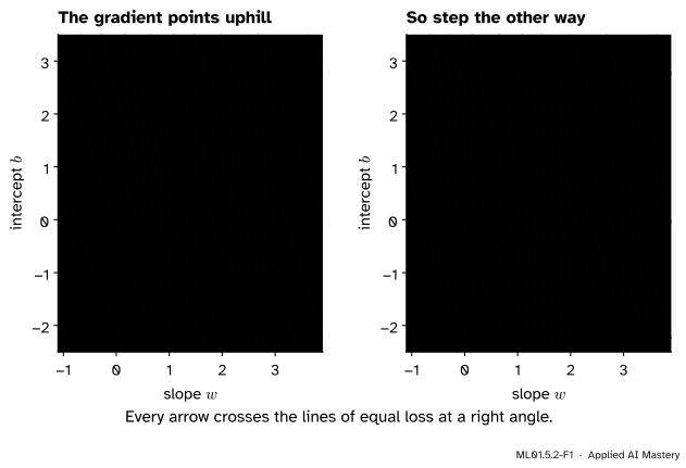
The gradient is not just a list. As an arrow on the map it has a meaning: it points in the direction in which the loss rises fastest. It points straight uphill.
ML01.5.2-F1
Left: the gradient at four places, pointing uphill. Right: the update moves the opposite way. The arrows are drawn at one twenty-fifth of the gradient’s true length, and each one crosses the contour lines at a right angle.
So the way down is the opposite arrow, \(-\nabla L\). Gradient descent computes the gradient where it stands, takes a short step against it, and repeats. The length of the step is set by a small positive number \(\eta\), the learning rate.
Build it up
Step 1. A partial derivative is the slope of a slice. Lesson 1 cut the bowl along \(b = 0\) and found the parabola \(L(w) = 7.5w^2 - 23.5w + 18.5\), whose slope is \(15w - 23.5\). That slope is \(\pd{L}{w}\) on the line \(b = 0\). At the point \((1, 0)\) it equals \(-8.5\).
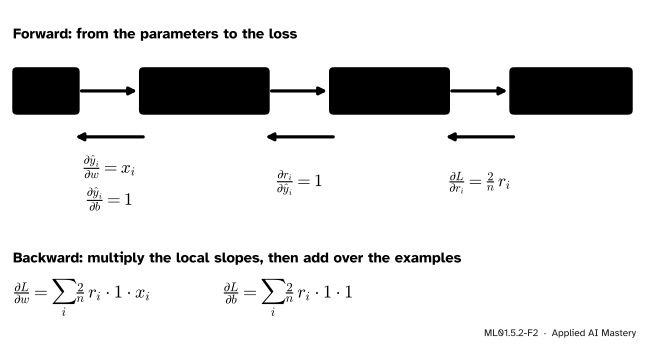
Step 2. The loss is a chain of three links. To get from the parameters to the loss you compute three things in turn: the prediction \(\hat{y}_i = w x_i + b\), the residual \(r_i = \hat{y}_i - y_i\), and the loss \(L = \frac{1}{n} \sum_i r_i^2\).
ML01.5.2-F2
The loss as a chain. Going forward computes the loss. Going backward, each link contributes one simple slope, and the chain rule multiplies them.
Step 3. The chain rule multiplies the slopes of the links. A small nudge to \(w\) changes the prediction \(x_i\) times as much. The residual changes by the same amount as the prediction. The loss changes \(\frac{2}{n} r_i\) times as much as the residual. Multiply the three, and add up over the examples, because \(w\) acts on the loss through every one of them.
Step 4. Step against the gradient, both parameters at once.
\[
w \leftarrow w - \eta\, \pd{L}{w}, \qquad b \leftarrow b - \eta\, \pd{L}{b} .
\]
Both slopes are measured at the current point, and only then are both parameters changed.
Step 5. Repeat. The new point has a new gradient. Compute it and step again. The path that results is a run of gradient descent.
The formal statement
NoteResult: the gradient of the mean squared error
For \(L(w, b) = \frac{1}{n} \sum_{i=1}^{n} (\hat{y}_i - y_i)^2\) with \(\hat{y}_i = w x_i + b\),
In words: the slope along \(w\) is twice the average of residual times input, and the slope along \(b\) is twice the average residual.
Derivation of \(\pd{L}{w}\). Write \(r_i = \hat{y}_i - y_i = w x_i + b - y_i\).
\[
\begin{aligned}
& \pd{L}{w} \\
&= \pd{}{w} \Big( \frac{1}{n} \sum_i r_i^2 \Big) \\
&= \frac{1}{n} \sum_i \pd{}{w} \big( r_i^2 \big) \\
&\quad\ \small\text{(a constant factor and a sum} \\
&\quad\ \small\text{pass through the derivative)} \\
&= \frac{1}{n} \sum_i 2\, r_i \cdot \pd{r_i}{w} \\
&\quad\ \small\text{(chain rule: the slope of a} \\
&\quad\ \small\text{square is twice the inside,} \\
&\quad\ \small\text{times the inside's slope)} \\
&= \frac{1}{n} \sum_i 2\, r_i \cdot \pd{}{w} \big( w x_i + b - y_i \big) \\
&= \frac{1}{n} \sum_i 2\, r_i \cdot x_i \\
&\quad\ \small\text{(} w x_i \text{ has slope } x_i \text{; } b \text{ and } y_i \\
&\quad\ \small\text{do not depend on } w \text{)} \\
&= \frac{2}{n} \sum_i (\hat{y}_i - y_i)\, x_i .
\end{aligned}
\]
Derivation of \(\pd{L}{b}\). The first three steps are the same with \(b\) in place of \(w\). Only the innermost slope differs: \(\pd{}{b}(w x_i + b - y_i) = 1\), because \(b\) has slope \(1\) in itself and the other two terms do not depend on \(b\). So
A check against lesson 1. Put \(b = 0\). Then \(\pd{L}{w} = \frac{2}{n} \sum_i (w x_i - y_i) x_i = 2 \cdot 7.5\, w - 2 \cdot 11.75 = 15w - 23.5\), the slope of the slice found there.
Why stepping against the gradient lowers the loss. For a small step \((\Delta w, \Delta b)\), the loss changes by about slope times distance in each direction:
\[
\Delta L \;\approx\; \pd{L}{w}\, \Delta w + \pd{L}{b}\, \Delta b .
\]
Choose the step \(\Delta w = -\eta\, \pd{L}{w}\) and \(\Delta b = -\eta\, \pd{L}{b}\). Then
A sum of squares is never negative, so for a small enough \(\eta\) the loss goes down, and it stays level only where both slopes are zero. “Small enough” is the catch, and it is the whole subject of lesson 3.
Where the gradient is zero. At the bottom of the bowl both slopes vanish. Using the averages from lesson 1, \(\pd{L}{b} = 2(2.5w + b - 4) = 0\) gives \(b = 4 - 2.5w\). Substituting into \(\pd{L}{w} = 2(7.5w + 2.5b - 11.75) = 0\) gives \(7.5w + 10 - 6.25w - 11.75 = 0\), so \(1.25w = 1.75\) and \(w = 1.4\). Then \(b = 4 - 3.5 = 0.5\): the least-squares line again.
Go deeper: why the gradient is the steepest direction, not just an uphill one
Write the step as a vector \(\vect{d} = (\Delta w, \Delta b)\). The first-order change in the loss is the dot product \(\nabla L \cdot \vect{d} = \norm{\nabla L}\, \norm{\vect{d}} \cos\theta\), where \(\theta\) is the angle between the step and the gradient. Among all steps of one fixed length, this is largest when \(\cos\theta = 1\), a step along the gradient, and most negative when \(\cos\theta = -1\), a step exactly against it. So \(\nabla L\) is the direction of steepest ascent and \(-\nabla L\) the direction of steepest descent.
When \(\cos\theta = 0\) the loss does not change to first order. Those are the steps along a contour line. That is why the gradient crosses every contour at a right angle.
Frontier note: the same chain, a billion parameters long
The backward pass in the chain diagram above is the whole idea of backpropagation. A deep network is a much longer chain of simple links. Deep-learning libraries keep track of the links as the loss is computed, then walk the chain backwards, multiplying local slopes, to get the slope of the loss with respect to every parameter at once. The update rule that follows is the one in this lesson, or a refinement of it.
Worked example
One full update by hand, from \((w, b) = (0, 0)\) with learning rate \(\eta = 0.05\).
At the start every prediction is \(0 \cdot x_i + 0 = 0\), so each residual is \(-y_i\).
Did the loss fall? Before the step it was \((4 + 9 + 25 + 36)/4 = 18.5\). The new line predicts \(1.575,\ 2.75,\ 3.925,\ 5.1\), so the residuals are \(-0.425,\ -0.25,\ -1.075,\ -0.9\) and
One step took the loss from \(18.5\) to \(0.552\).
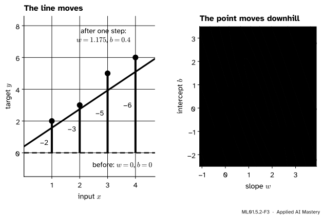
ML01.5.2-F3
The same update seen twice. Left: in data space, the flat starting line swings up towards the points. Right: on the loss map, the point jumps from the origin almost to the bottom of the valley. The short second arrow is the next step.
A second step from \((1.175, 0.4)\) works the same way. Its gradient is \((-3.875, -1.325)\), the new point is \((1.36875,\ 0.46625)\) and the loss falls to about \(0.064\). The gradient has shrunk, so the step has shrunk too, although \(\eta\) never changed. Gradient descent slows down by itself as the ground levels out.
Code
Gradient descent from scratch. The gradient function is the boxed result, line for line.
import numpy as npx = np.array([1.0, 2.0, 3.0, 4.0])y = np.array([2.0, 3.0, 5.0, 6.0])def loss(w, b):return np.mean((w * x + b - y) **2)def gradient(w, b): residual = w * x + b - y # y_hat - y, one entry per examplereturn2* np.mean(residual * x), 2* np.mean(residual)def gradient_descent(w, b, lr, steps):for _ inrange(steps): dw, db = gradient(w, b) # both slopes at the current point ... w, b = w - lr * dw, b - lr * db # ... then both parameters movereturn w, bprint("gradient at (0, 0):", np.round(gradient(0.0, 0.0), 3))for steps in [1, 2, 10, 100, 1000]: w, b = gradient_descent(0.0, 0.0, lr=0.05, steps=steps)print(f"after {steps:>4} steps: w = {w:.6f}, b = {b:.6f}, L = {loss(w, b):.6f}")
gradient at (0, 0): [-23.5  -8. ]
after    1 steps: w = 1.175000, b = 0.400000, L = 0.552187
after    2 steps: w = 1.368750, b = 0.466250, L = 0.063737
after   10 steps: w = 1.406247, b = 0.481632, L = 0.050056
after  100 steps: w = 1.401608, b = 0.495274, L = 0.050004
after 1000 steps: w = 1.400000, b = 0.500000, L = 0.050000
The first two rows match the worked example. Before trusting a gradient you derived, test it. A finite-difference check measures each slope directly: nudge one parameter a little each way and divide the change in the loss by the distance.
def numerical_gradient(w, b, h=1e-5): dw = (loss(w + h, b) - loss(w - h, b)) / (2* h) db = (loss(w, b + h) - loss(w, b - h)) / (2* h)return dw, dbrng = np.random.default_rng(0)worst =0.0for _ inrange(100): w, b = rng.uniform(-3, 3, size=2) gap = np.abs(np.subtract(gradient(w, b), numerical_gradient(w, b))).max() worst =max(worst, gap)print(f"largest gap between the formula and the measurement at 100 points: {worst:.1e}")
largest gap between the formula and the measurement at 100 points: 2.6e-09
Last, the library answer. Fitting a line by least squares has an exact solution, so there is something to compare with. NumPy solves it directly, and scikit-learn wraps the same kind of solver in a model object.
from sklearn.linear_model import LinearRegressiondesign = np.column_stack([x, np.ones_like(x)]) # one column for w, one for b(w_exact, b_exact), *_ = np.linalg.lstsq(design, y, rcond=None)model = LinearRegression()model.fit(x.reshape(-1, 1), y) # one row per example, one column per featurew_gd, b_gd = gradient_descent(0.0, 0.0, lr=0.05, steps=2000)print(f"np.linalg.lstsq: w = {w_exact:.6f}, b = {b_exact:.6f}")print(f"LinearRegression: w = {model.coef_[0]:.6f}, b = {model.intercept_:.6f}")print(f"gradient descent: w = {w_gd:.6f}, b = {b_gd:.6f} (2000 steps)")
np.linalg.lstsq:   w = 1.400000, b = 0.500000
LinearRegression:  w = 1.400000, b = 0.500000
gradient descent:  w = 1.400000, b = 0.500000   (2000 steps)
All three agree on \(w = 1.4\), \(b = 0.5\). Look again at the table of steps, though. Two steps brought the slope within \(0.04\) of its final value, yet after 100 steps the third decimal place is still wrong. The run falls into the valley at once and then creeps along its floor. Lesson 3 explains why, and how to fix it.
Explore
This module’s interactive, the gradient descent explorer, is in lesson 3. Its read-out shows the gradient at every step, so you can watch both slopes shrink towards zero as the path nears the bottom.
Pitfalls
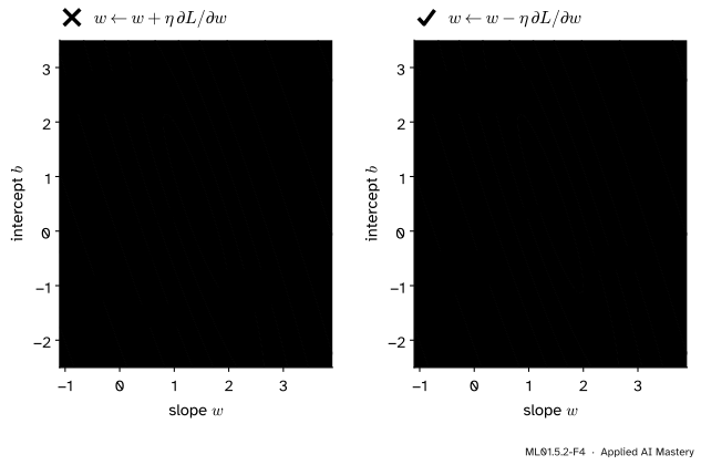
ML01.5.2-F4
Wrong beside right. One sign is the whole difference between climbing and descending.
“Add the gradient to the parameters.”
The gradient points uphill. Adding it climbs, and the loss grows at every step, as on the left of the figure. The update subtracts. If a training loss rises steadily from the very first step, check this sign before anything else.
“The negative gradient points at the minimum.”
It points straight downhill from where you stand, at a right angle to the contour line. In a long valley that is mostly across the valley, not along it. At \((w, b) = (-0.3, 2)\) the downhill direction and the direction of the minimum are \(58^\circ\) apart. From \((0, 0)\) the two happen to agree almost exactly, which is why the worked example made such a good first step.
“Update \(w\), then use the new \(w\) to work out the slope for \(b\).”
Both slopes belong to one point, the current one. Compute both first, then change both. Updating one parameter and re-using it straight away is a different algorithm with a different path. In code, a tuple assignment such as w, b = w - lr * dw, b - lr * db keeps the update simultaneous.
“The constant in front of the loss does not matter.”
It does not move the minimum, but it scales the gradient. Many books define the loss with a factor \(\tfrac{1}{2}\), which cancels the \(2\) and halves every slope. The same \(\eta\) then takes steps half as long. When you copy a learning rate from a book or a library, check which loss it goes with.
Check yourself
Recall
1. What is the gradient of \(L(w, b)\)?
Show answer
The arrow made of the two partial derivatives, \(\nabla L = \big( \pd{L}{w}, \pd{L}{b} \big)\).
2. Write the two partial derivatives of the mean squared error of a line.
3. Which way does the gradient point on the loss map, and how does it meet the contour lines?
Show answer
Straight uphill, in the direction where the loss rises fastest. It crosses the contour lines at a right angle.
4. State the update rule and name \(\eta\).
Show answer
\(w \leftarrow w - \eta\, \pd{L}{w}\) and \(b \leftarrow b - \eta\, \pd{L}{b}\), both computed at the current point. \(\eta\) is the learning rate.
5. What is the gradient at the lowest point of the bowl? Is the loss zero there?
Show answer
The gradient is \((0, 0)\). The loss need not be zero: for the running example it is \(0.05\).
Exercises
1.★ Compute the gradient at \((w, b) = (1, 0)\) by hand, then make one update with \(\eta = 0.05\).
Show solution
The predictions are \(1, 2, 3, 4\), so the residuals are \(-1, -1, -2, -2\), with sum \(-6\). The products \(r_i x_i\) are \(-1, -2, -6, -8\), with sum \(-17\). So \(\pd{L}{w} = \frac{2}{4} \cdot (-17) = -8.5\) and \(\pd{L}{b} = \frac{2}{4} \cdot (-6) = -3\). The update gives \(w = 1 + 0.05 \cdot 8.5 = 1.425\) and \(b = 0 + 0.05 \cdot 3 = 0.15\). The value \(-8.5\) is the slope of the slice \(b = 0\) at \(w = 1\) from lesson 1.
2.★★ A curved model adds a third parameter: \(\hat{y}_i = w x_i + b + c\, x_i^2\). The loss is still the mean squared error. Derive \(\pd{L}{c}\).
Show solution
Only the innermost link changes. With \(r_i = w x_i + b + c\, x_i^2 - y_i\),
The pattern holds for every parameter: twice the average of the residual times whatever multiplies that parameter in the prediction.
3.★★★ For any dataset, set both partial derivatives to zero and solve for \(w\) and \(b\). Write \(\bar{x}\), \(\bar{y}\), \(\overline{xy}\) and \(\overline{x^2}\) for the averages of \(x_i\), \(y_i\), \(x_i y_i\) and \(x_i^2\). Check your formulas on the running example.
Show solution
\(\pd{L}{b} = \frac{2}{n} \sum_i (w x_i + b - y_i) = 2\,(w \bar{x} + b - \bar{y})\). Setting it to zero gives \(b = \bar{y} - w \bar{x}\).
\(\pd{L}{w} = \frac{2}{n} \sum_i (w x_i + b - y_i)\, x_i = 2\,(w\, \overline{x^2} + b\, \bar{x} - \overline{xy})\). Setting it to zero and substituting \(b\):
For the running example \(\bar{x} = 2.5\), \(\bar{y} = 4\), \(\overline{xy} = 11.75\) and \(\overline{x^2} = 7.5\), so \(w = (11.75 - 10)/(7.5 - 6.25) = 1.75/1.25 = 1.4\) and \(b = 4 - 1.4 \cdot 2.5 = 0.5\). The formula needs \(\overline{x^2} \neq \bar{x}^2\), which holds unless every \(x_i\) is the same.
Summary card
The gradient points uphill, so step the other way.
ML01.5.2-F1
Uphill arrow, downhill step.
Gradient.\(\nabla L = \big( \pd{L}{w}, \pd{L}{b} \big)\), with \(\pd{L}{w} = \frac{2}{n} \sum_i (\hat{y}_i - y_i)\, x_i\) and \(\pd{L}{b} = \frac{2}{n} \sum_i (\hat{y}_i - y_i)\).
Update rule.\(w \leftarrow w - \eta\, \pd{L}{w}\) and \(b \leftarrow b - \eta\, \pd{L}{b}\), both from the current point.
Why it works.\(\Delta L \approx -\eta \big[ (\pd{L}{w})^2 + (\pd{L}{b})^2 \big] \le 0\) for a small enough \(\eta\).
By hand. From \((0, 0)\) with \(\eta = 0.05\): gradient \((-23.5, -8)\), new point \((1.175, 0.4)\), loss \(18.5 \to 0.552\).
Always test. A derived gradient should match finite differences.
Sources and next steps
Sources. Each was opened and checked against this lesson on 12 November 2026.
Tengyu Ma and Andrew Ng, CS229 Lecture Notes, Stanford University, Section 1.1 (LMS algorithm). Gives the update \(\theta_j := \theta_j - \alpha\, \partial J / \partial \theta_j\), performed simultaneously for all \(j\), calls \(\alpha\) the learning rate, and derives the partial derivative for a single training example line by line. Their cost carries a factor \(\tfrac{1}{2}\), so their gradient has no factor \(2\).
Ian Goodfellow, Yoshua Bengio and Aaron Courville, Deep Learning, MIT Press, 2016, Section 4.3. States that the gradient points directly uphill and the negative gradient directly downhill, and gives the steepest-descent step as equation 4.5, with the learning rate as a positive scalar that sets the size of the step.
Aston Zhang, Zachary Lipton, Mu Li and Alexander Smola, Dive into Deep Learning, Section 12.3.2. Uses the first-order expansion (12.3.6) to show that the negative gradient is the direction of steepest descent, and writes the update as equation (12.3.7). For the note on backpropagation: Section 2.5 says that a deep-learning framework builds a graph of how each value depends on others and works backwards through it with the chain rule, and Section 5.3.3 defines backpropagation as traversing the network in reverse order, from the output to the input layer, according to the chain rule.
Google, Machine Learning Crash Course, Linear regression: Gradient descent. Its worked maths uses the same convention as this lesson: a mean over the examples, with the factor \(2\) kept in both derivatives.
scikit-learn 1.9 documentation, LinearRegression, which fits by ordinary least squares and stores the result in coef_ and intercept_; and the NumPy 2.5 manual, numpy.linalg.lstsq, which returns the least-squares solution of a linear system.