A loss is a function of the model’s parameters, not of the data. See the mean squared error of a line as a parabola in one parameter and a bowl in two, and learn why training a model means walking downhill on that surface.
Explain why the loss is a function of the parameters w and b, with the data held fixed.
Compute the mean squared error of a candidate line by hand from its residuals.
Derive that the loss is a quadratic in w when b is held fixed, and find its lowest point.
Read a contour map of the loss and match points on it to lines through the data.
Use the sign of the slope of the loss to decide which way to move a parameter.
In review. The maths and code on this page are checked by automated tests on every change, but an independent reader has not signed it off yet. Spot a mistake or a confusing step? Tell us.
The question
Four points and a ruler. You can lay the ruler down in endlessly many ways, and each way is a candidate line. How could a computer find the best one without trying them all? Almost every model you will meet, from this line to a network with billions of weights, is trained by answering that one question.
Intuition
The running example of this module is as small as a learning problem gets. There are four examples, \((1, 2)\), \((2, 3)\), \((3, 5)\) and \((4, 6)\), and the model is a straight line, \(\hat{y} = wx + b\). The slope\(w\) and the intercept\(b\) are its two parameters.
A loss is a single number that says how badly a line misses the examples. A good line has a small loss and a bad line a large one.
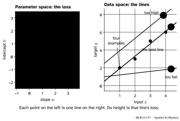
Here is the shift in point of view that the whole module rests on. The four examples never change. What changes is the pair \((w, b)\). So the loss is not a property of the data. It is a function of the parameters: put in a pair \((w, b)\), get out one number, \(L(w, b)\).
A function of two numbers can be drawn as a landscape. Lay the pairs \((w, b)\) out on a flat map, slope to the east and intercept to the north, and let the loss be the height of the ground at each spot.
ML01.5.1-F1
The loss landscape of the running example. Left: every point of the map is one pair \((w, b)\), and the purple curves join pairs with the same loss. Right: the same three pairs drawn as lines. Line C fits best, so point C is the lowest of the three.
Point A is a line that is too flat, so it sits high up. Point B has the right slope but floats above the data, so it is high too. Point C is the line that fits best, and it is the lowest point of the whole map.
Training a model means finding that lowest point. Nobody hands the computer the map. It stands at one spot, feels which way the ground slopes, and takes a step downhill. That is gradient descent, and the next three lessons build it. This lesson builds the ground it walks on.
Build it up
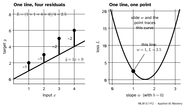
Step 1. One line gives one number. Take the candidate \(w = 1\), \(b = 0\), the line \(\hat{y} = x\). For each example, the residual is the prediction minus the target, \(\hat{y}_i - y_i\). The line predicts \(1, 2, 3, 4\) and the targets are \(2, 3, 5, 6\), so the residuals are \(-1, -1, -2, -2\). Square each one, so that misses above and below both count, and take the average:
This average is the mean squared error. One line went in and one number came out.
Step 2. Slide the slope and the number traces a curve. Keep \(b = 0\) and change \(w\). Each value of \(w\) is a different line through the origin, with its own loss. Plot the loss against \(w\) and the points join into a smooth curve.
ML01.5.1-F2
Left: the line \(w = 1\), \(b = 0\) and its four residuals, which average to a loss of \(2.5\). Right: that line is the single orange point. Every other slope gives another point, and together they make the purple curve.
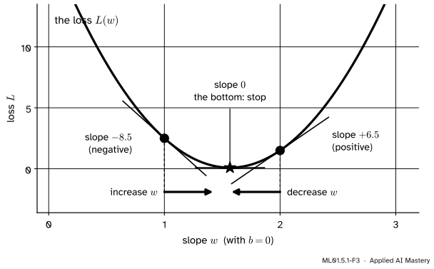
Step 3. The slope of the curve says which way is down. Stand on the curve at \(w = 1\). The curve falls to the right there: its slope is negative. So increasing \(w\) lowers the loss. At \(w = 2\) the curve rises to the right: its slope is positive, and decreasing \(w\) lowers the loss. At the very bottom the curve is flat, the slope is zero, and there is nowhere lower to go.
ML01.5.1-F3
Downhill in one picture. Where the slope of the loss is negative, move \(w\) up. Where it is positive, move \(w\) down. Where it is zero, stop.
That rule is the idea of the whole module: move each parameter against the sign of the slope. You never need to see the whole curve. The slope where you stand is enough.
Step 4. Free the intercept and the curve becomes a bowl. With \(b = 0\) we only looked at lines through the origin. Let \(b\) vary as well and every pair \((w, b)\) gets a height. The surface is a bowl, and the left panel of the first figure is that bowl seen from above. Each purple contour line joins the pairs that share one loss, the way a line on a hiking map joins places at one height. The curve of Step 2 is a single slice through the bowl, the cut along \(b = 0\).
For these four examples the bowl is long and narrow, more a valley than a soup bowl. Lesson 3 explains why, and what it costs.
The formal statement
NoteDefinition: mean squared error of a line
For \(n\) examples \((x_i, y_i)\) and the model \(\hat{y}_i = w x_i + b\), the mean squared error is
The parameters are the inputs of this function. The data and the targets are constants inside it. This module always divides by \(n\) and uses no factor of one half. Some books write \(\tfrac{1}{2}\) in front. That halves every loss value and moves no minimum.
Result 1: with \(b\) fixed, the loss is a quadratic in \(w\). Group each residual as \(w x_i - (y_i - b)\) and expand the square:
That is \(A w^2 - B w + C\), a quadratic, and its graph is a parabola. The number \(A\) is an average of squares, so it is positive unless every \(x_i\) is zero. A positive \(A\) means the parabola opens upward and has exactly one lowest point.
For the running example with \(b = 0\): \(\sum x_i^2 = 1 + 4 + 9 + 16 = 30\), \(\sum x_i y_i = 2 + 6 + 15 + 24 = 47\) and \(\sum y_i^2 = 4 + 9 + 25 + 36 = 74\). So \(A = 30/4 = 7.5\), \(B = 2 \cdot 47 / 4 = 23.5\) and \(C = 74/4 = 18.5\):
Result 2: where the bottom is. Complete the square. For any quadratic with \(A > 0\),
\[
\begin{aligned}
A w^2 - B w + C &= A \Big( w - \frac{B}{2A} \Big)^2 \\
&\quad {} + C - \frac{B^2}{4A} .
\end{aligned}
\]
To check, expand the right-hand side: \(A w^2 - 2A \cdot \tfrac{B}{2A}\, w + A \cdot \tfrac{B^2}{4A^2} + C - \tfrac{B^2}{4A} = A w^2 - B w + C\). A square is never negative, so the loss is smallest when the square is zero, at \(w = B / (2A)\). Here that is \(w = 23.5 / 15 \approx 1.567\), where the loss is \(18.5 - 23.5^2 / 30 \approx 0.092\).
Result 3: the slope at any point. Differentiating term by term,
\[
\begin{aligned}
\frac{dL}{dw} &= 2A\,w - B = 15\,w - 23.5 \\
&\quad\ \small\text{(for } b = 0\text{)}
\end{aligned}
\]
At \(w = 1\) this is \(-8.5\) and at \(w = 2\) it is \(+6.5\), the two slopes drawn in the figure above. It is zero exactly at \(w = 23.5/15\), the bottom.
Result 4: with both parameters free. Expand the full square, \((w x_i + b - y_i)^2 = w^2 x_i^2 + 2wb\,x_i + b^2 - 2w\,x_i y_i - 2b\,y_i + y_i^2\), and average each term. The averages of \(x_i^2\), \(x_i\), \(x_i y_i\), \(y_i\) and \(y_i^2\) are \(7.5\), \(2.5\), \(11.75\), \(4\) and \(18.5\), so
Every term has degree two or less. A surface like that with a single lowest point is a bowl, and its contour lines are ellipses. Here the lowest point is \(w = 1.4\), \(b = 0.5\), where \(L = 0.05\), as the proof below shows.
Go deeper: a proof, with school algebra only, that the lowest point is (1.4, 0.5)
Complete the square twice, first in \(b\) and then in \(w\). Collect the terms that contain \(b\): \(b^2 + 5wb - 8b = b^2 + 2b\,(2.5w - 4)\). Adding and subtracting \((2.5w - 4)^2\) gives
Two squares plus \(0.05\). Neither square can be negative, so \(L \ge 0.05\) everywhere. Equality needs both squares to be zero: \(w = 1.4\), and then \(b = 4 - 2.5 \cdot 1.4 = 0.5\). So the bowl has one lowest point, and no other spot on the map is as low.
The same form gives the contour lines. With \(u = b + 2.5w - 4\) and \(v = w - 1.4\), a fixed loss above \(0.05\) means \(u^2 + 1.25\,v^2\) equals a fixed positive number. That is the equation of an ellipse in \(u\) and \(v\). Changing back to \(w\) and \(b\) only shifts and shears it, and a sheared ellipse is still an ellipse.
Worked example
Compute the loss of four lines through the origin by hand, and find where the bottom lies.
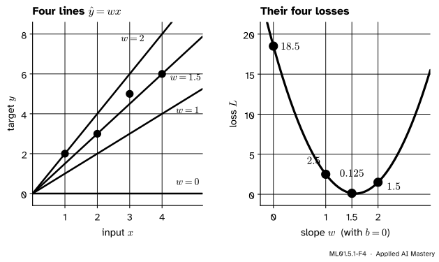
Take \(b = 0\) and the slopes \(w = 0, 1, 1.5, 2\). For each, the predictions are \(w \cdot 1\), \(w \cdot 2\), \(w \cdot 3\), \(w \cdot 4\). Subtract the targets \(2, 3, 5, 6\) to get the residuals, then average their squares.
\(w\)
Residuals \(\hat{y}_i - y_i\)
Loss \(L\)
\(0\)
\(-2,\)\(-3,\)\(-5,\)\(-6\)
\(\frac{4 + 9 + 25 + 36}{4}\)\(= 18.5\)
\(1\)
\(-1,\)\(-1,\)\(-2,\)\(-2\)
\(\frac{1 + 1 + 4 + 4}{4}\)\(= 2.5\)
\(1.5\)
\(-0.5,\)\(0,\)\(-0.5,\)\(0\)
\(\frac{0.25 + 0 + 0.25 + 0}{4}\)\(= 0.125\)
\(2\)
\(0,\)\(1,\)\(1,\)\(2\)
\(\frac{0 + 1 + 1 + 4}{4}\)\(= 1.5\)
ML01.5.1-F4
The table as a picture. Each line on the left is one orange point on the right, at the height the table gives.
The formula from Result 1 agrees with the table. At \(w = 1.5\) it gives \(7.5 \cdot 2.25 - 23.5 \cdot 1.5 + 18.5 = 16.875 - 35.25 + 18.5 = 0.125\).
The loss falls from \(18.5\) to \(2.5\) to \(0.125\), then rises to \(1.5\). The smallest value in the table is at \(w = 1.5\) and the losses on both sides of it are larger, so the bottom of the parabola lies between its two neighbours, \(w = 1\) and \(w = 2\). The slope narrows that down without a search: \(15 \cdot 1.5 - 23.5 = -1\) is negative, so the bottom is to the right of \(1.5\), and \(15 \cdot 2 - 23.5 = +6.5\) is positive, so it is to the left of \(2\). Result 2 gives the exact spot, \(w \approx 1.567\).
Code
First the loss from scratch, checked against the table.
import numpy as npx = np.array([1.0, 2.0, 3.0, 4.0])y = np.array([2.0, 3.0, 5.0, 6.0])def loss(w, b):"""Mean squared error of the line y_hat = w * x + b.""" y_hat = w * x + breturn np.mean((y_hat - y) **2)for w in [0.0, 1.0, 1.5, 2.0]:print(f"w = {w:<4} b = 0 L = {loss(w, 0.0):.3f}")
w = 0.0  b = 0   L = 18.500
w = 1.0  b = 0   L = 2.500
w = 1.5  b = 0   L = 0.125
w = 2.0  b = 0   L = 1.500
Next, the quadratic of Result 1. Its three coefficients come straight from the data.
A = np.mean(x **2) # coefficient of w squaredB =2* np.mean(x * y) # coefficient of w, for b = 0C = np.mean(y **2)w_bottom = B / (2* A)print("A, B, C =", A, B, C)print(f"bottom of the slice b = 0: w = {w_bottom:.4f}, L = {loss(w_bottom, 0.0):.4f}")print("slope at w = 1 and w = 2:", 2* A *1- B, 2* A *2- B)
A, B, C = 7.5 23.5 18.5
bottom of the slice b = 0: w = 1.5667, L = 0.0917
slope at w = 1 and w = 2: -8.5 6.5
Now the whole landscape. The crude way to find its lowest point is to compute the loss on a grid of pairs \((w, b)\) and take the smallest. The library way is one call to a least-squares routine.
ws = np.arange(-1.0, 4.0, 0.1)bs = np.arange(-2.5, 3.5, 0.1)grid = np.array([[loss(w, b) for w in ws] for b in bs]) # one row per value of brow, col = np.unravel_index(grid.argmin(), grid.shape)print(f"lowest grid point: w = {ws[col]:.1f}, b = {bs[row]:.1f}, L = {grid[row, col]:.3f}")slope, intercept = np.polyfit(x, y, deg=1) # least-squares lineprint(f"np.polyfit: w = {slope:.4f}, b = {intercept:.4f}, L = {loss(slope, intercept):.4f}")
lowest grid point: w = 1.4, b = 0.5, L = 0.050
np.polyfit:        w = 1.4000, b = 0.5000, L = 0.0500
The grid needed 3,000 evaluations of the loss to find two numbers. With a million parameters a grid is hopeless, and for most models no formula like the one behind polyfit exists. Walking downhill needs neither.
Explore
This module’s interactive, the gradient descent explorer, is in lesson 3. It shows this same contour map, with the line for each point beside it, and lets you walk the landscape step by step.
Pitfalls
ML01.5.1-F5
Wrong beside right. The best line through the origin is the bottom of one slice. The bottom of the bowl is somewhere else, and lower.
“I found the best \(w\), so now I just find the best \(b\).”
The best slope depends on the intercept. With \(b = 0\) the best slope is \(1.567\) and the loss is \(0.092\). The best pair is \(w = 1.4\), \(b = 0.5\), with loss \(0.05\). Tuning one parameter with the other frozen lands on the bottom of a slice. To reach the bottom of the bowl, both must move.
“The loss curve is a picture of the data.”
Its horizontal axis is \(w\), not \(x\). A point on it is not an example. It is a whole line. The data appear nowhere on the loss landscape, yet they shaped all of it: change one example and the entire surface shifts.
“The best line has zero loss.”
Only if the examples lie exactly on a line. These four do not, so the lowest loss any line can reach is \(0.05\). Training finds the lowest point of the landscape, whatever its height.
“Downhill means making \(w\) smaller.”
Downhill refers to the loss, not to the parameter. At \(w = 1\) the way down is to increase \(w\). At \(w = 2\) it is to decrease it. The sign of the slope decides, and it changes from place to place.
Check yourself
Recall
1. When we call the loss a function, what is its input and what stays fixed?
Show answer
The input is the parameters, here the pair \((w, b)\). The examples \((x_i, y_i)\) stay fixed.
2. What is a residual, and how does the mean squared error combine the residuals?
Show answer
A residual is a prediction minus its target, \(\hat{y}_i - y_i\). The mean squared error squares each residual and takes the average: \(L = \frac{1}{n} \sum_i (\hat{y}_i - y_i)^2\).
3. With \(b\) held fixed, what shape is the graph of \(L\) against \(w\), and why does it have one lowest point?
Show answer
A parabola, because \(L(w) = A w^2 - B w + C\) is a quadratic. The coefficient \(A = \frac{1}{n} \sum_i x_i^2\) is positive, so the parabola opens upward.
4. What does one contour line on the loss map join together?
Show answer
All the pairs \((w, b)\) that have the same loss, like a height line on a hiking map.
5. The slope of the loss at your current \(w\) is negative. Which way should \(w\) move, and when should it stop?
Show answer
Increase \(w\): the loss falls to the right. Stop where the slope is zero.
Exercises
1.★ Compute the loss of the line \(\hat{y} = 2x - 1\) on the four examples by hand.
Show solution
The predictions are \(1, 3, 5, 7\). The residuals are \(1 - 2 = -1\), \(3 - 3 = 0\), \(5 - 5 = 0\) and \(7 - 6 = 1\). Their squares are \(1, 0, 0, 1\), so \(L = 2/4 = 0.5\). Check with Result 4: \(7.5 \cdot 4 + 5 \cdot 2 \cdot (-1) + 1 - 23.5 \cdot 2 - 8 \cdot (-1) + 18.5 = 30 - 10 + 1 - 47 + 8 + 18.5 = 0.5\).
2.★★ Fix the intercept at \(b = 0.5\). Find the quadratic \(L(w)\), its lowest point and the loss there.
Show solution
Use Result 1 with \(y_i - b = 1.5, 2.5, 4.5, 5.5\). Then \(A = 7.5\) as before. \(\sum_i x_i (y_i - b) = 1.5 + 5 + 13.5 + 22 = 42\), so \(B = 2 \cdot 42 / 4 = 21\). \(\sum_i (y_i - b)^2 = 2.25 + 6.25 + 20.25 + 30.25 = 59\), so \(C = 59/4 = 14.75\). Hence
\[
L(w) = 7.5\,w^2 - 21\,w + 14.75 .
\]
The bottom is at \(w = B/(2A) = 21/15 = 1.4\), with loss \(14.75 - 21^2/30 = 14.75 - 14.7 = 0.05\). Completing the square, \(L(w) = 7.5\,(w - 1.4)^2 + 0.05\). This slice passes through the lowest point of the whole bowl, and lesson 3 uses it.
3.★★★ Now fix the slope at \(w = 1.4\) and let \(b\) vary. Show that \(L(b) = (b - 0.5)^2 + 0.05\). Then compare the coefficient of \(b^2\) here with the coefficient of \(w^2\) in exercise 2. What does the comparison say about the shape of the bowl?
Show solution
Write each residual as \(b + (1.4\,x_i - y_i)\), and call \(d_i = 1.4\,x_i - y_i\), which gives \(-0.6, -0.2, -0.8, -0.4\). Then \((b + d_i)^2 = b^2 + 2b\,d_i + d_i^2\). Averaging,
The coefficient of \(b^2\) is \(1\), whatever the data. The coefficient of \(w^2\) is \(7.5\). So moving \(w\) by some amount away from the bottom raises the loss \(7.5\) times as much as moving \(b\) by the same amount. The bowl is much steeper along \(w\) than along \(b\), which is one reason its contour lines are stretched. The term \(5\,wb\) tilts the valley and stretches them further, as lesson 3 measures.
Summary card
The loss is a landscape over the parameters, and training walks downhill on it.
ML01.5.1-F1
Each point is one line.
Loss.\(L(w, b) = \frac{1}{n} \sum_i (w x_i + b - y_i)^2\): a function of \(w\) and \(b\), with the data fixed.
One parameter. With \(b\) fixed, \(L(w) = A w^2 - B w + C\) with \(A = \frac{1}{n} \sum_i x_i^2 > 0\): a parabola with its bottom at \(w = B/(2A)\).
Two parameters. A bowl. For the running example, \(L = 7.5w^2 + 5wb + b^2 - 23.5w - 8b + 18.5\), lowest at \((1.4,\ 0.5)\) where \(L = 0.05\).
Downhill. Slope negative: increase the parameter. Slope positive: decrease it. Slope zero: stop.
Sources and next steps
Sources. Each was opened and checked against this lesson on 12 November 2026.
Tengyu Ma and Andrew Ng, CS229 Lecture Notes, Stanford University. Chapter 1 defines the least-squares cost function of linear regression, and Section 1.1 states that it is a convex quadratic function with one global optimum and shows its elliptical contours. Their cost is \(\tfrac{1}{2}\) times a sum, where this module uses \(\tfrac{1}{n}\) times a sum. The lowest point is the same.
Google, Machine Learning Crash Course, Linear regression: Loss. Defines the mean squared error as the average of the squared differences over \(N\) examples, the convention used here.
Google, Machine Learning Crash Course, Linear regression: Gradient descent. Its loss-surface figures put the weight and the bias on two axes and the loss on the third, and the text states that the loss functions of linear models always produce a convex surface.
Ian Goodfellow, Yoshua Bengio and Aaron Courville, Deep Learning, MIT Press, 2016, Section 4.3. States that a function can be reduced by moving its input in small steps with the opposite sign of the derivative, and illustrates it in Figure 4.1.