A fitted line hands you a few numbers: a slope, an intercept, an R squared. Learn what a coefficient means and which units it carries, derive R squared as the share of variance the line explains, and use residual plots, outliers and Anscombe’s quartet to see when the numbers mislead.
Interpret a slope and an intercept in words, with their units, and say how they change when the units of x change.
Explain why a coefficient in a model with several features describes a change with the other features held fixed.
Derive R squared as one minus the residual sum of squares over the total sum of squares, and compute it by hand.
Read a residual plot, and say what a curve or a lone far point in it suggests.
Show with Anscombe’s quartet and with one outlier how the same fitted line can describe very different data.
In review. The maths and code on this page are checked by automated tests on every change, but an independent reader has not signed it off yet. Spot a mistake or a confusing step? Tell us.
The question
A report says: “each extra hour of study adds 9 points to the quiz score (\(R^2 = 0.95\))”. Two numbers, and they sound like the end of the story. What do they claim? What do they leave out? And how can four datasets that look nothing alike give the same line and the same \(R^2\)? A model is only useful if you can tell when to believe it.
From the last lesson
1. State the normal equations, and say what they mean for the residuals.
Show answer
\(\mat{X}\T\mat{X}\,\vect{w} = \mat{X}\T\vect{y}\), which is the same as \(\mat{X}\T\vect{r} = \vect{0}\): the residuals are perpendicular to every column of \(\mat{X}\).
2. What does the column of ones in \(\mat{X}\) do?
Show answer
Its weight is the bias. Every row multiplies it by \(1\), so it is added to every prediction.
Intuition
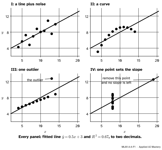
In 1973 the statistician F. J. Anscombe published four datasets of eleven points each. Feed any of them to the formulas of this module and the same numbers come out: mean of \(x\)\(9\), mean of \(y\)\(7.5\), fitted line \(\hat{y} = {0.5x + 3}\), and \(R^2 = 0.67\).
ML01.4.4-F1
Anscombe’s quartet. The four datasets share their fitted line and their \(R^2\). Only the first is what those numbers suggest.
Dataset I is a line plus noise, and the summary describes it fairly. Dataset II is a smooth curve. Dataset III is an exact line with one wild point that has pulled the fit off it. In dataset IV one point alone decides the slope.
Very different data can share one summary. So this lesson has two halves. First read the numbers properly. Then look at what they leave out.
Build it up
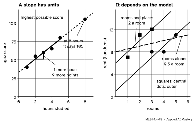
Step 1. A slope has units. The study table of course P01 has five students, with hours studied \(2, 4, 5, 1, 3\) and quiz scores \(55, 65, 80, 40, 60\). Its least-squares line is \(\hat{y} = {9x + 33}\). The slope is \(9\)points per hour: of two students who differ by one hour of study, the model expects the one who studied longer to score \(9\) points more. The intercept, \(33\)points, is the prediction for zero hours.
Step 2. Change the units and the number changes. With study time in minutes the same line reads \(\hat{y} = {0.15x' + 33}\), because \(9\) points per hour is \(9/60 = 0.15\) points per minute. The predictions are untouched. So the size of a coefficient says nothing about how much a feature matters until the features share a scale (lesson ML01.3.3).
Step 3. A coefficient belongs to a model. For the six flats of the last lesson, the fit with both features was \(\hat{y} = {2x_1 + 5x_2 + 1}\): two hundred a month for each extra room, for flats in the same kind of place. Fit the rent to the rooms alone and the slope is only \(0.5\).
ML01.4.4-F2
Left: the slope of the study line, and what happens when the line is pushed beyond the data. Right: the same feature in two models. With the place in the model, a room is worth \(2\). Without it, \(0.5\).
Why the difference? In this table the central flats are small and dear. A model that sees only the rooms mixes two things: more rooms raise the rent, but more rooms also go with being outside the centre, which lowers it. The coefficient \(2\) compares flats that differ in rooms and not in place. The coefficient \(0.5\) compares flats that differ in rooms and in whatever comes along with rooms. They answer different questions.
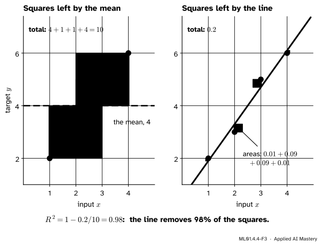
Step 4. How good is the fit? Compare the line with the laziest model: ignore \(x\) and always predict the mean of \(y\). The share of that baseline’s squared error which the line removes is called \(R^2\). For the four points the baseline’s loss is \(2.5\) and the line’s is \(0.05\), so \(R^2 = {1 - 0.05/2.5} = 0.98\).
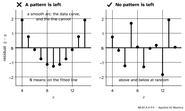
Step 5. Look at what is left. Plot each residual against its \(x\). This residual plot is the fitted line laid flat, with the misses standing on it. If a line is the right shape for the data, the residuals scatter above and below zero with no pattern. A curve in the plot says the data bend and the line cannot. One residual far from the rest marks an outlier.
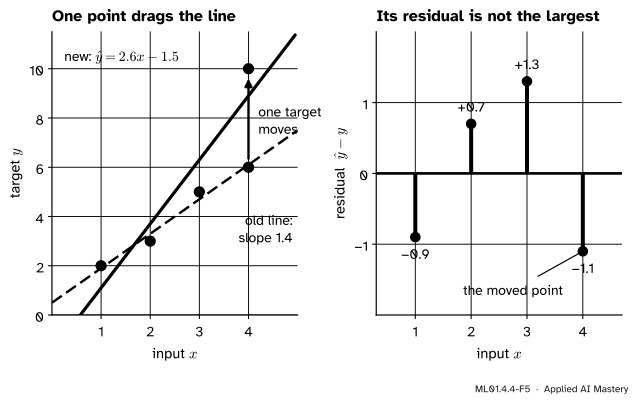
Step 6. One point can drag the line. Change the last target of the four points from \(6\) to \(10\). The best line swings from slope \(1.4\) to slope \(2.6\) to chase it.
ML01.4.4-F5
One changed target and the fit it produces. The line bends towards the far point until that point’s own residual, \(-1.1\), is smaller in size than its neighbour’s, \(+1.3\).
The moved point does not have the largest residual. It sits at the end of the range of \(x\), where a point has the most pull on the slope: it has leverage. The line gives way to it, and the damage shows up in the other residuals.
The formal statement
NoteDefinition: R squared
For targets \(y_i\) with mean \(\bar{y}\) and predictions \(\hat{y}_i\), the total sum of squares and the residual sum of squares are
Dividing both sums by \(n\) gives the loss of the mean and the loss of the model, so \(R^2 = {1 - L_{\text{model}} / L_{\text{mean}}}\), as in Step 4. A perfect model has \(R^2 = 1\). A model exactly as good as the mean has \(R^2 = 0\), and a worse one a negative \(R^2\).
Result 1: the split of the total. For a least-squares fit with a bias,
To derive it, write \(r_i = \hat{y}_i - y_i\) and go from the mean to a target in two steps, by way of the prediction: \(y_i - \bar{y} = {(\hat{y}_i - \bar{y})} - r_i\). Square it:
Sum over the examples. The first and last terms give \(SS_{\text{reg}}\) and \(SS_{\text{res}}\). The middle term vanishes. For a line, \(\hat{y}_i = {w x_i + b}\), so
by the two balances of lesson 2. With several features the same holds, because \(\sum_i r_i \hat{y}_i = (\mat{X}\vect{w})\T\vect{r} = \vect{w}\T\mat{X}\T\vect{r} = 0\) and the column of ones gives \(\sum_i r_i = 0\).
So \(R^2 = {1 - SS_{\text{res}}/SS_{\text{tot}}} = SS_{\text{reg}}/SS_{\text{tot}}\). Divided by \(n\), \(SS_{\text{tot}}\) is the variance of the targets and \(SS_{\text{reg}}\) the variance of the predictions, whose mean is also \(\bar{y}\). That is why \(R^2\) is called the share of variance explained. Both are sums of squares, so for a least-squares fit on its own data, \({0 \le R^2 \le 1}\).
Result 2: with one feature, \(R^2\) is the squared correlation. Since \(b = {\bar{y} - w\bar{x}}\), each prediction satisfies
\[
\begin{aligned}
\hat{y}_i - \bar{y} &= w x_i + b - \bar{y} \\
&= w\,(x_i - \bar{x}) .
\end{aligned}
\]
Square both sides, add over the examples and divide by \(n\):
The correlation of \(x\) and \(y\) is \(s_{xy}/(s_x s_y)\), so \(R^2\) is its square. For the four points, \(R^2 = {1.75^2 / (1.25 \cdot 2.5)} = {3.0625 / 3.125} = 0.98\).
Result 3: changing the units of \(x\). Let \(x_i' = k x_i\) with \(k \neq 0\). Every deviation from the mean is multiplied by \(k\), so the covariance becomes \(k\, s_{xy}\) and the variance \(k^2 s_x^2\). The new slope and intercept are
\[
\begin{aligned}
w' x_i' + b' &= \frac{w}{k} \cdot k x_i + b \\
&= w x_i + b .
\end{aligned}
\]
The slope absorbs the change of units. The residuals do not change, so neither does \(R^2\).
Worked example
Compute \(R^2\) for the four points and their least-squares line, by hand.
The line is \(\hat{y} = {1.4x + 0.5}\) and the mean of the targets is \(\bar{y} = 4\). The columns tot, res and reg hold each example’s \((y_i - \bar{y})^2\), \((\hat{y}_i - y_i)^2\) and \((\hat{y}_i - \bar{y})^2\): for the first example \((-2)^2\), \((-0.1)^2\) and \((-2.1)^2\).
\(x_i\)
\(y_i\)
\(\hat{y}_i\)
tot
res
reg
\(1\)
\(2\)
\(1.9\)
\(4\)
\(0.01\)
\(4.41\)
\(2\)
\(3\)
\(3.3\)
\(1\)
\(0.09\)
\(0.49\)
\(3\)
\(5\)
\(4.7\)
\(1\)
\(0.09\)
\(0.49\)
\(4\)
\(6\)
\(6.1\)
\(4\)
\(0.01\)
\(4.41\)
sum
\(10\)
\(0.2\)
\(9.8\)
ML01.4.4-F3
The two sums of squares as areas: \(10\) for the mean and \(0.2\) for the line.
The split holds: \(9.8 + 0.2 = 10\). So \(R^2 = {1 - 0.2/10} = 9.8/10 = 0.98\). The line removes \(98\%\) of the squared error that the mean leaves behind.
Now with the outlier of Step 6. The targets \(2, 3, 5, 10\) have mean \(5\) and deviations \(-3, -2, 0, 5\). With the deviations \(-1.5, -0.5, 0.5, 1.5\) of \(x\), the products sum to \(4.5 + 1 + 0 + 7.5 = 13\), so \(w = 13/5 = 2.6\) and \(b = 5 - 2.6 \cdot 2.5 = -1.5\). The predictions are \(1.1, 3.7, 6.3, 8.9\) and the residuals \(-0.9, 0.7, 1.3, -1.1\). Then
An \(R^2\) of \(0.89\) still sounds good. Yet the slope has nearly doubled, and only the residuals show it.
Code
\(R^2\) from scratch, on the examples of this lesson.
import numpy as npdef fit_line(x, y):"""Least-squares slope and intercept (lesson 2).""" w = np.mean((x - x.mean()) * (y - y.mean())) / np.var(x)return w, y.mean() - w * x.mean()def r_squared(y, y_hat): ss_res = np.sum((y_hat - y) **2) ss_tot = np.sum((y - y.mean()) **2)return1- ss_res / ss_totx = np.array([1.0, 2.0, 3.0, 4.0])y = np.array([2.0, 3.0, 5.0, 6.0])w, b = fit_line(x, y)print(f"four points: y_hat = {w:.1f}x + {b:.1f} R^2 = {r_squared(y, w * x + b):.4f}")hours = np.array([2.0, 4.0, 5.0, 1.0, 3.0])score = np.array([55.0, 65.0, 80.0, 40.0, 60.0])w_h, b_h = fit_line(hours, score)w_m, b_m = fit_line(60* hours, score) # the same study time, in minutesprint(f"study table: y_hat = {w_h:.0f}x + {b_h:.0f} R^2 = {r_squared(score, w_h * hours + b_h):.4f}")print(f"in minutes: slope {w_m:.2f}, intercept {b_m:.0f}, prediction at 8 hours: {w_h *8+ b_h:.0f}")y_out = np.array([2.0, 3.0, 5.0, 10.0]) # one target changed from 6 to 10w_o, b_o = fit_line(x, y_out)print(f"with outlier: y_hat = {w_o:.1f}x - {-b_o:.1f} R^2 = {r_squared(y_out, w_o * x + b_o):.4f}"f" residuals {np.round(w_o * x + b_o - y_out, 2)}")
four points:    y_hat = 1.4x + 0.5    R^2 = 0.9800
study table:    y_hat = 9x + 33     R^2 = 0.9529
in minutes:     slope 0.15, intercept 33, prediction at 8 hours: 105
with outlier:   y_hat = 2.6x - 1.5    R^2 = 0.8895    residuals [-0.9  0.7  1.3 -1.1]
In scikit-learn, r2_score takes the targets and the predictions, and every regressor has a score method that returns \(R^2\). Here they are on the six flats.
rooms alone:       slope 0.50, intercept 8.00, R^2 = 0.116
rooms and central: weights [2. 5.], intercept 1.00, R^2 = 0.814
plus a column of noise: R^2 = 0.826
A column of random numbers raised \(R^2\) from \(0.81\) to \(0.83\): the last pitfall explains why. Now Anscombe’s quartet. The numbers agree, and three checks show what a plot would.
x123 = np.array([10, 8, 13, 9, 11, 14, 6, 4, 12, 7, 5], dtype=float)quartet = {"I": (x123, np.array([8.04, 6.95, 7.58, 8.81, 8.33, 9.96, 7.24, 4.26, 10.84, 4.82, 5.68])),"II": (x123, np.array([9.14, 8.14, 8.74, 8.77, 9.26, 8.10, 6.13, 3.10, 9.13, 7.26, 4.74])),"III": (x123, np.array([7.46, 6.77, 12.74, 7.11, 7.81, 8.84, 6.08, 5.39, 8.15, 6.42, 5.73])),"IV": (np.array([8, 8, 8, 8, 8, 8, 8, 19, 8, 8, 8], dtype=float), np.array([6.58, 5.76, 7.71, 8.84, 8.47, 7.04, 5.25, 12.50, 5.56, 7.91, 6.89])),}for name, (xs, ys) in quartet.items(): slope, intercept = fit_line(xs, ys)print(f"{name:<4} y_hat = {slope:.2f}x + {intercept:.2f} R^2 = {r_squared(ys, slope * xs + intercept):.2f}")xs, ys = quartet["II"] # a curve: a parabola fits it exactlyprint(f"II with a squared term: R^2 = {r_squared(ys, np.polyval(np.polyfit(xs, ys, 2), xs)):.4f}")xs, ys = quartet["III"] # drop the one far pointkeep = ys <10print("III without its outlier: slope %.3f, intercept %.2f"% fit_line(xs[keep], ys[keep]))xs, ys = quartet["IV"]print("IV without its far point: variance of x =", np.var(xs[xs <19]))
I    y_hat = 0.50x + 3.00   R^2 = 0.67
II   y_hat = 0.50x + 3.00   R^2 = 0.67
III  y_hat = 0.50x + 3.00   R^2 = 0.67
IV   y_hat = 0.50x + 3.00   R^2 = 0.67
II with a squared term: R^2 = 1.0000
III without its outlier: slope 0.345, intercept 4.01
IV without its far point: variance of x = 0.0
Dataset II needs a squared term. Dataset III without its outlier is the line \(\hat{y} = {0.345x + 4.01}\), not \(0.5x + 3\). In dataset IV without the far point every \(x\) is \(8\), the variance is zero, and no slope can be computed.
Explore
In the line fitter of lesson 1, press Show best fit: the read-out gives the \(R^2\) of the best-fit line. Then drag the last point, at \(x = 4\), up to the top of the picture: Step 6 on a smaller scale. The dashed line swings after it, its slope rising from \(1.4\) to \(1.85\), yet \(R^2\) only falls from \(0.98\) to \(0.97\).
Pitfalls
ML01.4.4-F4
Residual plots of Anscombe’s datasets II (left) and I (right). Same line, same \(R^2\). Only the plot on the left says that a line is the wrong shape.
“\(R^2\) is high, so a line is the right model.”
\(R^2\) measures how much of the scatter the line removes, not whether the data are straight. Anscombe’s curve has the same \(R^2\) as his line plus noise. Plot the residuals: a pattern in them is the model’s missing piece.
“The slope says what will happen if I change \(x\).”
The slope describes differences between the examples in this data: students who studied an hour longer scored \(9\) points more, on average. It does not say that a student who adds an hour will gain \(9\) points, because students who study longer may differ in other ways too. Getting from “goes with” to “causes” takes more than a fit (course S06).
“The line holds for any \(x\).”
The line was fitted between \(1\) and \(5\) hours. At \(8\) hours it predicts \(9 \cdot 8 + 33 = 105\) points in a quiz marked out of \(100\). Predicting outside the range of the data is extrapolation, and nothing in the fit vouches for it. That includes the intercept when \(x = 0\) is far from the data.
“Adding a feature raised \(R^2\), so the model is better.”
On the data used for fitting, \(R^2\) cannot fall when a column is added: the old fit is still available, with a weight of zero on the new column. Even random numbers raised it above. Judge a model on data it was not fitted to (module ML01.2), where \(R^2\) can fall and can even be negative.
Check yourself
Recall
1. In the line \(\hat{y} = {9x + 33}\), with \(x\) in hours and \(y\) in quiz points, what do \(9\) and \(33\) mean?
Show answer
The predicted score is \(9\) points higher for each extra hour of study, and \(33\) points for zero hours.
2. If \(x\) is measured in minutes instead of hours, what happens to the slope, the intercept and the predictions?
Show answer
The slope is divided by \(60\), from \(9\) to \(0.15\). The intercept and every prediction stay the same.
3. Define \(R^2\), and say what the values \(1\) and \(0\) mean.
Show answer
\(R^2 = {1 - SS_{\text{res}}/SS_{\text{tot}}}\): one minus the model’s squared error over that of always predicting the mean. \(1\) means every prediction is exact, \(0\) just as good as the mean.
4. What does the residual plot of a good fit look like, and what does a curve in it mean?
Show answer
Residuals scattered above and below zero with no pattern. A curve means the data bend in a way the model cannot follow.
5. What do Anscombe’s four datasets have in common, and what is the lesson?
Show answer
The same means, fitted line \(\hat{y} = {0.5x + 3}\) and \(R^2 = 0.67\), though one is a line with noise, one a curve, one has an outlier and one has a slope set by a single point. The numbers of a fit do not show its shape: look at the data and the residuals.
Exercises
1.★ For the study table, the line \(\hat{y} = {9x + 33}\) has a mean squared error of \(8\), and the scores have a variance of \(170\). Compute \(R^2\). Then predict the score for \(6\) hours of study and say how far you trust it.
Show solution
\(R^2 = {1 - 8/170} = 162/170 \approx 0.953\). (Means work as well as sums, because the \(n\) cancels.) The line removes about \(95\%\) of the squared error of always guessing \(60\).
For \(6\) hours the line predicts \(9 \cdot 6 + 33 = 87\). The data run from \(1\) to \(5\) hours, so this is an extrapolation: a possible score, but no student in the table tells us that the straight trend continues. By \(8\) hours the line gives an impossible \(105\).
2.★★ For the six flats, with rooms \(3, 4, 5, 1, 2, 3\) and rents \(8, 8, 11, 7, 11, 12\), compute \(R^2\) for the model with rooms alone, \(\hat{y} = {0.5x_1 + 8}\), and for the model \(\hat{y} = {2x_1 + 5x_2 + 1}\), whose residuals are \(-1, 1, 0, 1, -1, 0\).
Show solution
The mean rent is \(57/6 = 9.5\). The deviations are \(-1.5\), \(-1.5\), \(1.5\), \(-2.5\), \(1.5\), \(2.5\), so \(SS_{\text{tot}} = 2.25 + 2.25 + 2.25 + 6.25 + 2.25 + 6.25 = 21.5\).
Rooms alone. The predictions are \(9.5, 10, 10.5, 8.5, 9, 9.5\) and the residuals \(1.5, 2, -0.5, 1.5, -2, -2.5\), so \(SS_{\text{res}} = 2.25 + 4 + 0.25 + 2.25 + 4 + 6.25 = 19\) and \(R^2 = {1 - 19/21.5} \approx 0.12\).
Rooms alone explain about \(12\%\) of the variance of the rents, rooms and place together about \(81\%\).
3.★★★ The split of Result 1 needs a least-squares fit. Show that without one, \(R^2\) can be negative, by computing it for the constant prediction \(\hat{y} = 6\) on the four points. Which step of the proof that \({R^2 \ge 0}\) fails?
Show solution
The residuals of \(\hat{y} = 6\) are \(6 - 2 = 4\), then \(3\), \(1\) and \(0\), so \(SS_{\text{res}} = 16 + 9 + 1 + 0 = 26\). With \(SS_{\text{tot}} = 10\),
\[
R^2 = 1 - \frac{26}{10} = -1.6 .
\]
A negative \(R^2\) means the model is worse than always predicting the mean. The proof that \(R^2 \ge 0\) used \(\sum_i r_i = 0\) to remove the middle term of the split. Here the residuals sum to \(8\), so the middle term stays. On new data a fitted model is in the same position: nothing forces its residuals there to balance.
Summary card
A fit gives numbers. Read them with their units, then look at what they leave out.
ML01.4.4-F1
Same line, four stories.
Slope. The change in the prediction per unit of \(x\), in units of \(y\) per unit of \(x\). With several features: with the others held fixed.
Units. If \(x' = kx\), then \(w' = w/k\), and \(b\), the predictions and \(R^2\) do not change.
R squared.\(R^2 = {1 - \dfrac{SS_{\text{res}}}{SS_{\text{tot}}}} = \dfrac{SS_{\text{reg}}}{SS_{\text{tot}}}\), the share of variance explained. With one feature, the squared correlation.
Four points.\(SS_{\text{tot}} = 10\), \(SS_{\text{res}} = 0.2\), \(R^2 = 0.98\).
Doubt. Plot the residuals. Watch for curves, outliers, points with leverage and extrapolation.
Sources and next steps
Sources. Each was opened and checked against this lesson on 12 November 2026.
F. J. Anscombe, Graphs in Statistical Analysis, The American Statistician 27(1), 1973, pages 17 to 21. The table of the four datasets, on page 19, and their shared summary: means \(9.0\) and \(7.5\), regression line \(y = {3 + 0.5x}\), multiple \(R^2 = 0.667\). It says that all but one point of dataset 3 lie close to the line \(y = {4 + 0.346x}\), and of dataset 4 that all the information about the slope “resides in one observation”. Anscombe’s residuals are observed minus fitted, the opposite sign to this course.
Mine Çetinkaya-Rundel and Johanna Hardin, Introduction to Modern Statistics, 2nd edition, Sections 7.2.3 to 7.3. Interpreting a slope and an intercept, extrapolation, \(R^2 = {1 - SSE/SST}\) as the proportion of variability explained, and leverage points.
scikit-learn 1.9 User Guide, R² score, Section 3.4.6.1, and the score method of LinearRegression. The formula used here; the best score is \(1.0\), it “can be negative”, and a constant model predicting the mean scores \(0.0\).
NIST/SEMATECH, e-Handbook of Statistical Methods, Section 4.4.4.1. Residual plots without systematic structure indicate a model that fits well; structure indicates that the form of the function can be improved.
OpenStax, Introductory Statistics 2e, Section 12.6. Points far from the others in the horizontal direction “may have a big effect on the slope of the regression line”.
Matplotlib 3.11 gallery, Anscombe’s quartet. The four datasets as arrays, matching Anscombe’s table.
Next.ML01.5.1 Loss as a landscape starts the next module: finding the best line by walking downhill, the method that still works when no formula exists.