A straight line with a slope and an intercept is the simplest model that predicts a number. Learn what a residual is, why the misses are squared before they are averaged, and how the mean squared error and the mean absolute error judge the same four points differently.
Write the prediction of a line as w times x plus b, and name the slope, the intercept and the residual.
Compute the mean squared error and the mean absolute error of a candidate line by hand.
Explain, with a line whose residuals sum to zero, why residuals are squared or made positive before they are averaged.
Derive that the best single guess under squared error is the mean, and under absolute error a median.
Compare how the two losses weigh one large miss against several small ones.
In review. The maths and code on this page are checked by automated tests on every change, but an independent reader has not signed it off yet. Spot a mistake or a confusing step? Tell us.
The question
Give two people a ruler and the same four points, and they will draw two different lines. Which is better? You cannot say until you fix a rule for scoring a line. That rule is the loss, and every model in machine learning is trained by making a loss small. So what is a fair way to score a line?
Intuition
The running example of this course is four invented points, small enough to work by hand: \((1, 2)\), \((2, 3)\), \((3, 5)\) and \((4, 6)\). Each is an example: an input \(x\) and the target\(y\) we would like to predict from it.
The simplest model that predicts a number from a number is a straight line,
\[
\hat{y} = w x + b .
\]
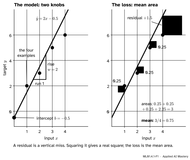
The hat marks a prediction, to keep it apart from the target \(y\). The line has two parameters. The slope\(w\) says how much the prediction rises when \(x\) grows by one. The intercept\(b\) is the prediction at \(x = 0\). Machine learning also calls them the weight and the bias. Each pair \((w, b)\) is one line.
ML01.4.1-F1
Left: one candidate line, \(\hat{y} = {2x - 0.5}\), and its two parameters. Right: how it is scored. Each vertical bar is a residual, the square on it has the squared residual as its area, and the loss is the mean of the four areas.
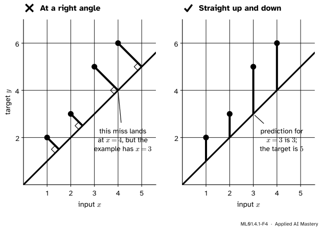
For each example, the gap between the prediction and the target is the residual. It is measured straight up and down, because the model is asked about that example’s own \(x\). A line that fits well has small squares.
Build it up
Step 1. Predictions. Take the candidate \(w = 2\), \(b = -0.5\). At \(x = 1, 2, 3, 4\) it predicts \(2 \cdot 1 - 0.5 = 1.5\), then \(3.5\), \(5.5\) and \(7.5\).
Step 2. Residuals. For each example, subtract the target from the prediction:
A positive residual means the line is too high at that \(x\), a negative one too low. This course always takes prediction minus target. Many statistics books take target minus prediction, which flips every sign. Both losses below ignore the sign.
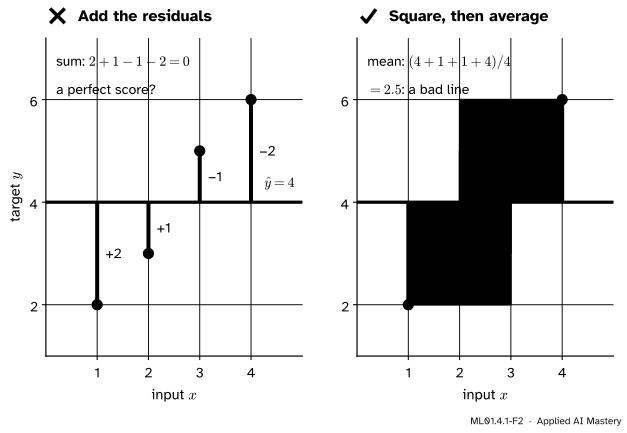
Step 3. One number for the whole line. Four residuals must become one score. Adding them up fails. Take the flat line \(\hat{y} = 4\), which ignores \(x\) altogether. Its residuals are \(4 - 2 = 2\), then \(1\), \(-1\) and \(-2\), and they add up to exactly zero: a perfect score for a line that misses every point.
ML01.4.1-F2
Left: added as they are, the misses above and below the flat line cancel. Right: squared first, nothing can cancel, and the line gets the poor score it deserves.
Step 4. Two repairs. Make the misses positive before averaging them. Take the absolute value of each residual and average: the mean absolute error. Or square each residual and average: the mean squared error. For the candidate line of Step 2 the mean absolute error is
The two happen to agree here, but they are made differently. The largest miss supplies half of the absolute total, \(1.5\) out of \(3\), and three quarters of the squared total, \(2.25\) out of \(3\).
Step 5. Why the square is usual. Three reasons, and one price.
Large misses count for more. A miss twice as large costs four times as much. Often one prediction that is badly off does more harm than two that are slightly off.
It is smooth. The curve \(r^2\) has a slope everywhere, so calculus can find the best line exactly (next lesson) and gradient descent has a clean step to take (module ML01.5). The curve \(\abs{r}\) has a corner at \(r = 0\).
It has one best answer. The squared error of a line has a single lowest point whenever the inputs are not all equal. The absolute error can have a flat stretch of equal answers.
The price. A single wild target can pull the whole line towards itself. Lesson 4 returns to that.
The formal statement
NoteDefinition: the line, its residuals and two losses
For \(n\) examples \((x_i, y_i)\), a line with slope \(w\) and intercept \(b\) predicts \(\hat{y}_i = {w x_i + b}\). The residual of example \(i\) is \(r_i = \hat{y}_i - y_i\). The mean squared error (MSE) and the mean absolute error (MAE) of the line are
In this course \(L\) means the mean squared error unless a lesson says otherwise, and a loss is always a mean: it divides by \(n\), with no factor of one half.
Result 1: scaling the misses. Multiply every residual by a number \(k\). Since \(\abs{k r_i} = \abs{k}\,\abs{r_i}\) and \((k r_i)^2 = k^2 r_i^2\), the factor comes out of each mean: the MAE is multiplied by \(\abs{k}\) and the MSE by \(k^2\). Doubling every miss doubles the MAE and quadruples the MSE.
Result 2: under squared error, the best single guess is the mean. Strip the model down to one number: predict the same value \(c\) for every example. Write \(\bar{y}\) for the mean of the targets and split each miss in two, \(c - y_i = {(c - \bar{y})} + {(\bar{y} - y_i)}\). Squaring gives
Average over the examples. The first term is the same for every \(i\). In the middle term the factor \(2(c - \bar{y})\) comes out, leaving the average of \(\bar{y} - y_i\), which is \(\bar{y} - \bar{y} = 0\). So
The second term does not contain \(c\). The first is a square, smallest when \(c = \bar{y}\). For the targets \(2, 3, 5, 6\) the mean is \(4\) and the second term is \({(4 + 1 + 1 + 4)}/4 = 2.5\), so the loss of the guess \(c\) is \((c - 4)^2 + 2.5\).
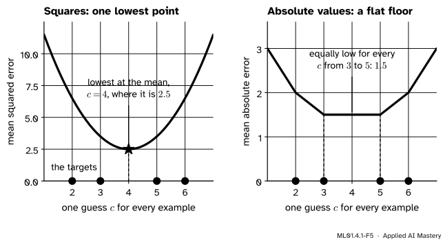
Result 3: under absolute error, the best single guess is a median. Move the guess \(c\) a little to the right, by \(\delta\), without crossing a target. Every target to the left of \(c\) is now \(\delta\) further away, and every target to the right is \(\delta\) closer. If \(l\) targets lie to the left (count one that sits exactly at \(c\)) and \(m\) to the right, the mean absolute error changes by \({\delta\,(l - m)/n}\). So it falls while more targets lie to the right, rises once more lie to the left, and is lowest where neither side holds more than half of the targets. That is a median. With the targets \(2, 3, 5, 6\), any \(c\) from \(3\) to \(5\) has \(2\) and \(3\) at or below it and \(5\) and \(6\) at or above it, so for all of them
The two losses in miniature. Squared error has a smooth bowl with one lowest point, at the mean. Absolute error is made of straight pieces with corners at the targets, and here it has a flat floor.
A line does the same job with two parameters instead of one. One more difference: the MSE is in squared units. If \(y\) is in metres, the MSE is in square metres, so an MSE and an MAE cannot be compared with each other. The square root of the MSE, the RMSE, is back in metres (lesson ML01.7.4).
Go deeper: where the square comes from if the noise is bell-shaped
Suppose each target is a point on a true line plus noise, \(y_i = w x_i + b + \varepsilon_i\), the \(\varepsilon_i\) being independent draws from a normal distribution with mean \(0\) and standard deviation \(\sigma\), whose density is \(p(\varepsilon) = \frac{1}{\sqrt{2\pi}\,\sigma} \exp\!\big(-\varepsilon^2 / (2\sigma^2)\big)\). For a candidate \((w, b)\) the noise must have been \(\varepsilon_i = y_i - w x_i - b\). By independence the density of all \(n\) targets is a product, and its logarithm is a sum:
The first term does not contain \(w\) or \(b\). The second is a negative constant times \(\sum_i r_i^2 = n L(w, b)\). So the line that makes the observed targets most probable is the one with the smallest mean squared error. With a noise density proportional to \(\exp(-\abs{\varepsilon}/s)\), the same steps leave \(-\frac{1}{s} \sum_i \abs{r_i}\): the smallest mean absolute error.
Worked example
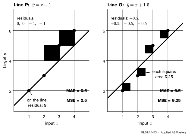
Two lines, scored both ways. Line P is \(\hat{y} = {x + 1}\). Line Q is \(\hat{y} = {x + 1.5}\), the same line moved up by a half. Their residuals \(\hat{y}_i - y_i\) and their two losses:
\(x_i\)
\(y_i\)
residual of P
residual of Q
\(1\)
\(2\)
\(0\)
\(0.5\)
\(2\)
\(3\)
\(0\)
\(0.5\)
\(3\)
\(5\)
\(-1\)
\(-0.5\)
\(4\)
\(6\)
\(-1\)
\(-0.5\)
MAE
\(0.5\)
\(0.5\)
MSE
\(0.5\)
\(0.25\)
ML01.4.1-F3
Line P is perfect on two points and off by \(1\) on two. Line Q is off by \(0.5\) on all four. The total length of the bars is the same. The total area of the squares is not.
The mean absolute error cannot tell the two lines apart: each has misses that add up to \(2\). The mean squared error prefers Q by a factor of two, because two misses of \(1\) cost \(2\) in squares and four misses of \(0.5\) cost \(4 \times 0.25 = 1\). Squaring rewards spreading the error evenly.
Each loss has its own best line. The next lesson derives the line with the lowest MSE, \(\hat{y} = {1.4x + 0.5}\). The line with the lowest MAE is a different one, \(\hat{y} = {\tfrac{4}{3}x + \tfrac{2}{3}}\), through the first and last points. Their residuals and their two losses:
\(x_i\)
\(y_i\)
\(1.4x + 0.5\)
\(\tfrac43 x + \tfrac23\)
\(1\)
\(2\)
\(-0.1\)
\(0\)
\(2\)
\(3\)
\(0.3\)
\(\tfrac13\)
\(3\)
\(5\)
\(-0.3\)
\(-\tfrac13\)
\(4\)
\(6\)
\(0.1\)
\(0\)
MAE
\(0.2\)
\(0.167\)
MSE
\(0.05\)
\(0.056\)
Each line wins on its own loss: the first has the lower MSE, the second the lower MAE, exactly \(\tfrac16\). The two best lines are close, but not the same. “The best line” always means “the best line for this loss”.
Go deeper: a proof that no line has a mean absolute error below one sixth
Write any line as \(\hat{y} = {{(\tfrac43 + u)}\,x + {(\tfrac23 + v)}}\). Its four residuals are
because \(3\abs{u} \ge u\). So the mean absolute error is at least \(\tfrac23 / 4 = \tfrac16\). Equality needs \(3\abs{u} = u\), so \(u = 0\), and then \(\abs{r_1} + \abs{r_4} = 2\abs{v} = 0\), so \(v = 0\). Only the line through the first and last points reaches \(\tfrac16\).
Code
First from scratch. Each function is one line of NumPy.
import numpy as npx = np.array([1.0, 2.0, 3.0, 4.0])y = np.array([2.0, 3.0, 5.0, 6.0])def predict(w, b):return w * x + bdef residuals(w, b):"""Prediction minus target, one number per example."""return predict(w, b) - ydef mse(w, b):return np.mean(residuals(w, b) **2)def mae(w, b):return np.mean(np.abs(residuals(w, b)))print("residuals of 2x - 0.5:", residuals(2.0, -0.5))print("plain sum of the residuals of the flat line y = 4:", residuals(0.0, 4.0).sum())lines = {"P: x + 1": (1.0, 1.0), "Q: x + 1.5": (1.0, 1.5),"1.4x + 0.5": (1.4, 0.5), "(4/3)x + 2/3": (4/3, 2/3)}for name, (w, b) in lines.items():print(f"{name:<13} MAE = {mae(w, b):.3f} MSE = {mse(w, b):.3f}")
residuals of 2x - 0.5: [-0.5  0.5  0.5  1.5]
plain sum of the residuals of the flat line y = 4: 0.0
P: x + 1       MAE = 0.500   MSE = 0.500
Q: x + 1.5     MAE = 0.500   MSE = 0.250
1.4x + 0.5     MAE = 0.200   MSE = 0.050
(4/3)x + 2/3   MAE = 0.167   MSE = 0.056
The numbers match the tables. The library versions take the targets and the predictions:
from sklearn.metrics import mean_absolute_error, mean_squared_errory_hat = predict(1.0, 1.5) # line Qprint("MAE:", mean_absolute_error(y, y_hat), " MSE:", mean_squared_error(y, y_hat))
MAE: 0.5 MSE: 0.25
Last, the one-number model of Results 2 and 3, with every guess from \(1\) to \(7\) in steps of \(0.01\).
guesses = np.linspace(1, 7, 601)mse_of = np.array([np.mean((c - y) **2) for c in guesses])mae_of = np.array([np.mean(np.abs(c - y)) for c in guesses])best = guesses[mse_of.argmin()]floor = guesses[np.isclose(mae_of, mae_of.min())]print(f"squared error: lowest at c = {best:.2f}, where it is {mse_of.min():.2f} (mean = {y.mean()})")print(f"absolute error: equally low from c = {floor.min():.2f} to {floor.max():.2f}, "f"where it is {mae_of.min():.2f} (median = {np.median(y)})")
squared error:  lowest at c = 4.00, where it is 2.50  (mean = 4.0)
absolute error: equally low from c = 3.00 to 5.00, where it is 1.50  (median = 4.0)
Explore
ML01.4-X1
Line fitter
Drag the line or its two knobs, or use the sliders, and make the squares as small as you can. Then press Show best fit to see how close you came. Drag a point, and the best line changes.
Look for two things. A miss twice as long covers four times the area. And when you drag one point far from the others, the best-fit line swings after it: the price of squaring.
Pitfalls
ML01.4.1-F4
Wrong beside right. The shortest path from a point to the line ends at a different \(x\). A residual uses the prediction for the example’s own \(x\), so it is vertical.
“The residual is the distance from the point to the line.”
It is the vertical gap, because the model answers one question: given this \(x\), what is \(y\)? For the line \(\hat{y} = x\) and the example \((3, 5)\) the residual is \(3 - 5 = -2\). The shortest path to the line is about \(1.41\) long and ends at \(x = 4\), an input this example never had.
“Add up the residuals. If the total is small, the line is good.”
Residuals above and below cancel. The flat line \(\hat{y} = 4\) has a total of \(0\) and a mean squared error of \(2.5\). A total of zero only says the line is too high as much as it is too low.
“There is one correct loss.”
A loss is a choice about which mistakes matter. Squared error chases large misses, so one wild value moves the fit a great deal: adding a fifth target of \(14\) to \(2, 3, 5, 6\) moves the mean from \(4\) to \(6\) and the median only from \(4\) to \(5\). Machine learning usually starts from squared error because it is smooth, and switches when the data call for it.
Check yourself
Recall
1. In \(\hat{y} = {wx + b}\), what does each of \(w\) and \(b\) do to the line?
Show answer
\(w\) is the slope: the prediction changes by \(w\) when \(x\) grows by one. \(b\) is the intercept: the prediction at \(x = 0\). Changing \(w\) tilts the line and changing \(b\) slides it up or down.
2. How is the residual of an example defined in this course, and what does its sign say?
Show answer
\(r_i = \hat{y}_i - y_i\), the prediction minus the target. Positive means the line is too high at that \(x\), negative means too low.
3. Why can the residuals not simply be added up?
Show answer
Positive and negative residuals cancel. The flat line \(\hat{y} = 4\) has residuals \(2, 1, -1, -2\), which sum to \(0\), though it misses every point.
4. Write the mean squared error and the mean absolute error of a line.
5. If one number must be guessed for every example, which guess is best under each loss?
Show answer
The mean of the targets under squared error. A median under absolute error, and there may be a whole stretch of equally good guesses.
Exercises
1.★ Compute the residuals, the MAE and the MSE of the line \(\hat{y} = {2x - 1}\) on the four points.
Show solution
The predictions are \(1, 3, 5, 7\). The residuals are \(1 - 2 = -1\), \(3 - 3 = 0\), \(5 - 5 = 0\) and \(7 - 6 = 1\). So \(\text{MAE} = {(1 + 0 + 0 + 1)}/4 = 0.5\) and \(L = {(1 + 0 + 0 + 1)}/4 = 0.5\). They agree because \(0\) and \(1\) equal their own squares.
2.★★ Someone mistypes the last target as \(10\) instead of \(6\). For the line \(\hat{y} = {1.4x + 0.5}\), compute both losses with the wrong target. By what factor has each grown?
Show solution
The predictions are \(1.9, 3.3, 4.7, 6.1\). Against the targets \(2, 3, 5, 10\) the residuals are \(-0.1,\ 0.3,\ -0.3\) and \(6.1 - 10 = -3.9\).
The sizes of the residuals add up to \({0.1 + 0.3 + 0.3 + 3.9} = 4.6\), so \(\text{MAE} = 4.6/4 = 1.15\). Before the typo it was \(0.2\), so it has grown by a factor of \(1.15 / 0.2 = 5.75\).
Their squares add up to \({0.01 + 0.09 + 0.09 + 15.21} = 15.4\), so \(L = 15.4/4 = 3.85\). Before it was \(0.05\), so it has grown by a factor of \(3.85 / 0.05 = 77\).
One bad value multiplied the absolute error by about \(6\) and the squared error by \(77\).
3.★★★ Five targets are \(2, 3, 5, 6\) and \(14\). One number \(c\) must be guessed for all of them. Find the best \(c\) and the loss it achieves, first under squared error and then under absolute error. Compare with the answers for the four targets without the \(14\).
Show solution
Squared error. By Result 2 the best guess is the mean, \({(2 + 3 + 5 + 6 + 14)}/5 = 30/5 = 6\). The loss there is the average squared deviation from the mean: \({(16 + 9 + 1 + 0 + 64)}/5 = 90/5 = 18\).
Absolute error. By Result 3 the best guess has no more than half of the targets on either side. With five targets that happens only at the middle one, \(c = 5\), with two targets on each side and a loss of \({(3 + 2 + 0 + 1 + 9)}/5 = 15/5 = 3\). Any move away from \(5\) goes away from three targets and towards only two, so the loss rises.
Comparison. Without the \(14\) the mean was \(4\) and every guess from \(3\) to \(5\) was a median, \(4\) being the usual choice. The new target moved the mean by \(2\), to \(6\), and the median by only \(1\), to \(5\).
Summary card
A line is scored by its misses, and squaring the misses decides which line wins.
Residual.\(r_i = \hat{y}_i - y_i\), measured vertically. Its sign says too high or too low.
Mean squared error.\(L(w, b) = \frac{1}{n} \sum_i {(\hat{y}_i - y_i)^2}\). Doubling the misses multiplies it by \(4\).
Mean absolute error.\(\frac{1}{n} \sum_i \abs{{\hat{y}_i - y_i}}\). Doubling the misses multiplies it by \(2\).
One-number model. Squared error is lowest at the mean, absolute error at a median.
Sources and next steps
Sources. Each was opened and checked against this lesson on 12 November 2026.
Google, Machine Learning Crash Course, Linear regression. Writes the model as \(y' = b + w_1 x_1\), with \(b\) the bias and \(w_1\) the weight.
Google, Machine Learning Crash Course, Linear regression: Loss. Defines the MAE and the MSE as averages over \(N\) examples, and states that “MSE moves the model more toward the outliers, while MAE doesn’t”.
Tengyu Ma and Andrew Ng, CS229 Lecture Notes, Stanford University. Chapter 1 defines the least-squares cost, with a factor \(\tfrac12\) and a sum where this course uses a mean. Section 1.3 shows that with independent Gaussian noise, least squares is maximum likelihood: the first “Go deeper” block.
scikit-learn 1.9 User Guide, Regression metrics, Sections 3.4.6.2 and 3.4.6.3. The formulas of mean_absolute_error and mean_squared_error.
Mine Çetinkaya-Rundel and Johanna Hardin, Introduction to Modern Statistics, 2nd edition, Section 7.1.3. Defines the residual as observed minus predicted, \(e_i = y_i - \hat{y}_i\), the opposite sign to this course.