The nearest-neighbour rule labels a new example by copying the label of the most similar example it has stored. Work it by hand with Euclidean distance on eight fruit, code it in NumPy and scikit-learn, and see the decision regions it draws.
Compute the Euclidean distance between two examples from their features, by hand and in NumPy.
Classify a new example with the 1-nearest-neighbour rule, showing every distance.
Derive the boundary between two stored examples, the straight line halfway between them, and sketch the decision regions of a small dataset.
Explain why the rule scores 100 percent on the examples it has stored and why that score says nothing about new examples.
In review. The maths and code on this page are checked by automated tests on every change, but an independent reader has not signed it off yet. Spot a mistake or a confusing step? Tell us.
The question
Someone hands you a fruit you have not seen before, and a tray of eight fruit that already carry labels. The simplest thing you can do is find the fruit on the tray that is most like yours and copy its label. What does “most like” mean in numbers? And can a program that only looks things up be said to have learned anything?
Intuition
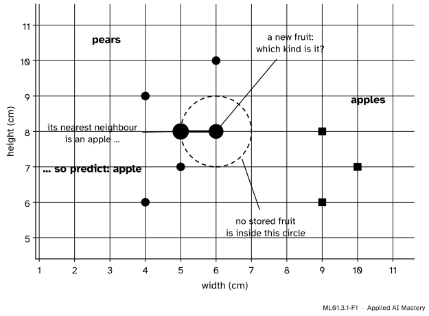
Describe each fruit by two features: its width and its height, in centimetres. Two numbers are a point on a plane, so the tray of labelled fruit becomes a picture. Pears are taller than they are wide. Apples are wider than they are tall. One apple on this tray is an odd one: it is 5 cm wide and 8 cm tall, and it sits among the pears.
ML01.3.1-F1
The nearest-neighbour rule. The stored fruit are points. The new fruit, marked “?”, is compared with every one of them. The closest is the apple one centimetre to its left, so the prediction is “apple”.
The nearest-neighbour rule has a single step: find the stored example that is closest to the new one, and predict its label. That closest example is the nearest neighbour.
Notice what is missing. Nothing was fitted. There are no parameters to adjust and no loss to lower. The “model” is the tray itself. All the work happens at the moment a question is asked.
Look again at the picture before going on. The rule says apple. Would you?
Build it up
Step 1. An example is a point. A fruit 6 cm wide and 8 cm tall is the point \({(6, 8)}\). We call the new fruit the query.
Step 2. “Most like” means “closest”. Two fruit with nearly the same width and nearly the same height are close together on the plane. So we need the distance between two points.
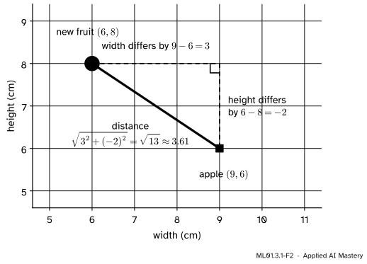
Step 3. Distance is the long side of a right-angled triangle. Walk from one point to the other in two legs: first sideways, by the difference in width, then up or down, by the difference in height. The two legs meet at a right angle, and the straight route is the third side.
ML01.3.1-F2
One distance. The widths differ by \(3\) and the heights by \({-2}\). Squaring removes the sign, and Pythagoras gives the straight-line distance, \({\sqrt{13} \approx 3.61}\) cm.
Step 4. Measure to every stored example and keep the smallest. Eight stored fruit means eight distances. The fruit with the smallest one is the nearest neighbour, and its label is the answer.
Step 5. Ask the question everywhere. Now imagine putting the query at every point of the plane in turn. Some places get the answer “pear” and others “apple”. The plane splits into decision regions, and the line where the answer changes is the decision boundary.
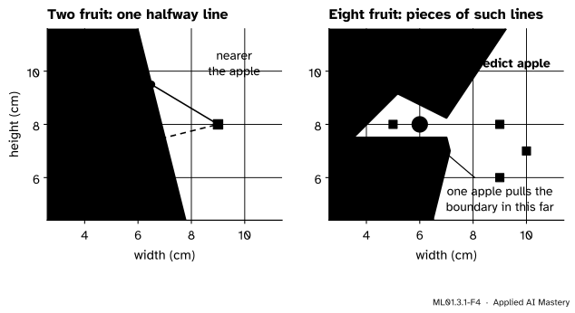
Start with just two stored fruit. A query is nearer to one or to the other, and the places where it is exactly as far from both form a straight line, halfway between them. With eight fruit, the boundary is made of pieces of such halfway lines.
ML01.3.1-F4
Left: two stored fruit share the plane along the line halfway between them. Right: eight stored fruit. The decision boundary is built from pieces of halfway lines, and the single apple at \({(5, 8)}\) drags apple territory deep in among the pears.
No one drew that boundary. It follows from where the stored fruit lie, and it can take any shape the data asks for. That is the rule’s strength. Its weakness is in the same picture: one odd fruit claims a whole wedge of the plane.
The formal statement
NoteDefinition: the nearest-neighbour rule
The training set holds \(n\) examples \({(\vect{x}_1, y_1), \dots, (\vect{x}_n, y_n)}\). Each \(\cdata{\vect{x}_i}\) is a list of \(d\) features and \(y_i\) is its label. The Euclidean distance between two points \(\vect{a}\) and \(\vect{b}\) is
Where the distance formula comes from. Take \({\vect{a} = (a_1, a_2)}\) and \({\vect{b} = (b_1, b_2)}\) on the plane, and the corner point \({(b_1, a_2)}\). The leg from \(\vect{a}\) to the corner is horizontal, with length \({\abs{b_1 - a_1}}\). The leg from the corner to \(\vect{b}\) is vertical, with length \({\abs{b_2 - a_2}}\). They meet at a right angle, so by Pythagoras
The last step uses the fact that a square does not care about sign. Taking the square root gives the formula with \({d = 2}\). With more features there are more legs, one per feature, and the same sum of squares is taken as the definition.
Fact 1: the square root can be skipped when ranking. Suppose two squared distances satisfy \({0 \le u < v}\). Could \({\sqrt{u} \ge \sqrt{v}}\)? Squaring both sides of that would give \({u \ge v}\), which is false. So \({\sqrt{u} < \sqrt{v}}\): the order of the squared distances is the order of the distances, and the nearest neighbour is the one with the smallest squared distance. By hand, that saves eight square roots.
Fact 2: the boundary between two stored points is a straight line. A query \(\vect{x}\) is equally far from \(\vect{a}\) and \(\vect{b}\) when the squared distances agree:
No square of \(x_1\) or \(x_2\) is left, and since \({\vect{a} \ne \vect{b}}\) their coefficients are not both zero, so this is the equation of a straight line. The midpoint \({\big(\tfrac{a_1 + b_1}{2}, \tfrac{a_2 + b_2}{2}\big)}\) lies on it. Put it into the left-hand side:
For the pear at \({(5, 7)}\) and the apple at \({(9, 8)}\) the line is \({2 \cdot 4\, x_1 + 2 \cdot 1\, x_2} = {145 - 74}\), that is \({8x_1 + 2x_2 = 71}\). The midpoint \({(7, 7.5)}\) satisfies it: \({56 + 15 = 71}\).
Fact 3: every stored example is classified correctly. If the query is a stored point \(\vect{x}_i\) itself, its distance to \(\vect{x}_i\) is \(0\), and its distance to any stored point in a different place is greater than \(0\). So its nearest neighbour is itself and the prediction is its own label. As long as no two stored examples sit on the same spot with different labels, the accuracy on the training set is exactly 100%.
Go deeper: the cells behind the regions
Give each stored point the set of all queries that are closer to it than to any other stored point. That set is its cell. The cells tile the plane, and the tiling is called a Voronoi diagram. The decision regions are unions of cells, and the decision boundary is made of the cell walls that have a pear on one side and an apple on the other.
Each wall is at a right angle to the segment joining its two points. Take two points \(\vect{x}\) and \(\vect{x}'\) on the halfway line, subtract their two equations and halve the result:
That is the dot product of \({\vect{b} - \vect{a}}\) with a direction along the line, and a dot product of zero means a right angle.
Frontier note: how good can so simple a rule be?
Better than it looks. Cover and Hart proved in 1967 that, for suitably smooth distributions and as the number of stored examples grows without limit, the rule’s error rate is at most twice the lowest that any classifier could reach on the same problem.
The rule is also alive in current systems. A search engine that stores documents as long lists of numbers, called embeddings, answers a query by finding the stored lists nearest to it. Lesson 4 explains why millions of points and hundreds of features both cause trouble.
Worked example
Classify the fruit that is 6 cm wide and 8 cm tall.
The query is \({(6, 8)}\). For each stored fruit, subtract the query’s width and height (the two differences, width first), square them and add. By Fact 1 the square root can wait until the end.
Stored fruit
Differences
Squared distance
pear \({(5, 7)}\)
\({-1,\ -1}\)
\({1 + 1} = 2\)
pear \({(6, 10)}\)
\({0,\ 2}\)
\({0 + 4} = 4\)
pear \({(4, 9)}\)
\({-2,\ 1}\)
\({4 + 1} = 5\)
pear \({(4, 6)}\)
\({-2,\ -2}\)
\({4 + 4} = 8\)
apple \({(5, 8)}\)
\({-1,\ 0}\)
\({1 + 0} = 1\)
apple \({(9, 8)}\)
\({3,\ 0}\)
\({9 + 0} = 9\)
apple \({(9, 6)}\)
\({3,\ -2}\)
\({9 + 4} = 13\)
apple \({(10, 7)}\)
\({4,\ -1}\)
\({16 + 1} = 17\)
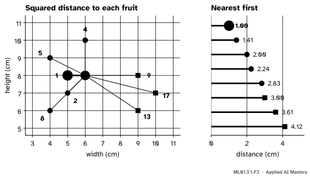
The square roots are in the figure.
ML01.3.1-F3
The table as a picture. Left: the squared distance from the query to each stored fruit. Right: the same eight fruit in order of distance. An apple comes first.
The smallest squared distance is \(1\), for the apple at \({(5, 8)}\). So
\[
\begin{aligned}
i^{*} &= \text{the apple at } (5, 8), \\
\cmodel{\hat{y}} &= \text{apple} .
\end{aligned}
\]
Now read the rest of the list. The next four neighbours are all pears, and the other three apples are the farthest fruit on the tray. The query is 6 cm wide and 8 cm tall: taller than wide, like a pear. The rule answered “apple” because of one fruit. Whether that fruit is a rare tall apple or a labelling mistake, the rule cannot tell, and it trusts it completely. Lesson 2 repairs this by asking more than one neighbour.
Code
From scratch first. The function does what the table did: one distance per stored fruit, then the smallest.
import numpy as npX = np.array([[5, 7], [6, 10], [4, 9], [4, 6], # four pears: width and height in cm [5, 8], [9, 8], [9, 6], [10, 7]]) # four applesy = np.array(["pear"] *4+ ["apple"] *4)query = np.array([6, 8])def euclidean(a, b):return np.sqrt(np.sum((a - b) **2))def nearest_neighbour(X, y, query): distances = np.array([euclidean(row, query) for row in X]) nearest = np.argmin(distances) # the index of the smallest distancereturn y[nearest], nearest, distanceslabel, nearest, distances = nearest_neighbour(X, y, query)for row, kind, d inzip(X, y, distances):print(f"{kind:5s}{str(tuple(int(v) for v in row)):8s} squared {d **2:3.0f} distance {d:.2f}")print("nearest:", tuple(int(v) for v in X[nearest]), "->", label)
NumPy can do all eight subtractions at once, and by Fact 1 the square root is not needed to find the winner.
squared = ((X - query) **2).sum(axis=1) # eight squared distances, no loopprint("squared distances:", squared)print("same winner without the square root:", np.argmin(squared) == np.argmin(np.sqrt(squared)))a, b = np.array([5, 7]), np.array([9, 8]) # the pear and the apple of Fact 2for point in [np.array([7.0, 7.5]), np.array([6.5, 9.5])]:print(point, "on the line:", 8* point[0] +2* point[1] ==71,"| distances:", euclidean(point, a).round(3), euclidean(point, b).round(3))
squared distances: [ 2  4  5  8  1  9 13 17]
same winner without the square root: True
[7.  7.5] on the line: True | distances: 2.062 2.062
[6.5 9.5] on the line: True | distances: 2.915 2.915
Both test points lie on the line \({8x_1 + 2x_2 = 71}\) and both are equally far from the two fruit. Now the library version. In scikit-learn the rule is KNeighborsClassifier with one neighbour. Its fit only stores the data.
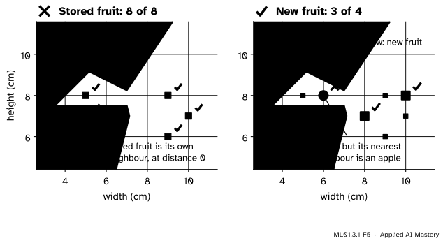
from sklearn.neighbors import KNeighborsClassifiermodel = KNeighborsClassifier(n_neighbors=1).fit(X, y)how_far, which = model.kneighbors([query])print("prediction:", model.predict([query])[0], "| neighbour index", which[0, 0], "at distance", how_far[0, 0])print("accuracy on the eight stored fruit:", model.score(X, y))X_new = np.array([[6, 8], [5, 10], [8, 7], [10, 8]]) # four fruit that were not on the trayy_new = np.array(["pear", "pear", "apple", "apple"])print("predictions for four new fruit:", model.predict(X_new))print("accuracy on the four new fruit:", model.score(X_new, y_new))
prediction: apple | neighbour index 4 at distance 1.0
accuracy on the eight stored fruit: 1.0
predictions for four new fruit: ['apple' 'pear' 'apple' 'apple']
accuracy on the four new fruit: 0.75
The library agrees with the hand calculation. It also shows Fact 3: the score on the stored fruit is a perfect \(1.0\). On four new fruit it is \(0.75\). The one mistake is our query, which was in truth a pear.
Explore
This module’s interactive, the neighbour explorer, is in lesson 2. Set its slider to \({k = 1}\) and you have this lesson’s rule: drag the query across the wedge round the odd apple and watch the answer flip.
Pitfalls
ML01.3.1-F5
Wrong beside right. Scoring the rule on the fruit it stored gives full marks, by Fact 3. Scoring it on fruit it has not stored shows what it can really do: here, three right out of four.
“It gets every training example right, so it must be a good classifier.”
By Fact 3 the rule scores 100% on its own training set even if half the labels were typed in wrongly. It is the lookup table of module ML01.2 with one addition: for an input it has not seen, it answers with the nearest entry. Only examples held back from the tray can measure how well that works.
“To get the distance, add up the differences.”
Differences have signs, and signs cancel. From the query \({(6, 8)}\) to the pear at \({(4, 9)}\) the differences are \({-2}\) and \(1\), which add to \({-1}\): a negative “distance”. Square each difference first, then add, then take the root. In NumPy that is np.sqrt(((a - b) ** 2).sum()), not (a - b).sum().
“The rule compares the new fruit with the typical pear and the typical apple.”
It compares the query with single stored examples, not with class averages. The average pear on the tray is at \({(4.75, 8)}\), only \(1.25\) cm from the query, and the average apple is \(2.37\) cm away, yet the rule says apple, because one apple is closer than any pear. Looking at single points lets the boundary take any shape. It also lets one odd point decide.
Check yourself
Recall
1. What does the nearest-neighbour rule do with a new example?
Show answer
It finds the stored example at the smallest distance from it and predicts that example’s label.
2. Write the Euclidean distance between \({(a_1, a_2)}\) and \({(b_1, b_2)}\).
Show answer
\(\sqrt{(a_1 - b_1)^2 + (a_2 - b_2)^2}\).
3. Why may you compare squared distances when you only want the nearest neighbour?
Show answer
The square root keeps order: if \({0 \le u < v}\) then \({\sqrt{u} < \sqrt{v}}\).
4. What is the boundary between the regions of two stored points?
Show answer
The straight line of points equally far from both. It passes through the midpoint of the segment joining them, at a right angle to it.
5. What accuracy does the rule reach on its own stored examples, and why?
Show answer
100%, provided no two stored examples coincide with different labels. Each one is at distance \(0\) from itself, so it is its own nearest neighbour.
Exercises
1.★ With the same eight stored fruit, classify a fruit 7 cm wide and 9 cm tall.
Show solution
The squared distances from \({(7, 9)}\) are: to \({(5, 7)}\), \({4 + 4 = 8}\); to \({(6, 10)}\), \({1 + 1 = 2}\); to \({(4, 9)}\), \({9 + 0 = 9}\); to \({(4, 6)}\), \({9 + 9 = 18}\); to \({(5, 8)}\), \({4 + 1 = 5}\); to \({(9, 8)}\), \({4 + 1 = 5}\); to \({(9, 6)}\), \({4 + 9 = 13}\); to \({(10, 7)}\), \({9 + 4 = 13}\). The smallest is \(2\), for the pear at \({(6, 10)}\). The prediction is pear.
2.★★ Find the halfway line between the pear at \({(5, 7)}\) and the apple at \({(5, 8)}\). Which part of the boundary in the regions figure is it?
Show solution
With \({\vect{a} = (5, 7)}\) and \({\vect{b} = (5, 8)}\), Fact 2 gives \({2(5 - 5)\,x_1 + 2(8 - 7)\,x_2} = {(25 + 64) - (25 + 49)}\), that is \({2x_2 = 15}\). The line is \({x_2 = 7.5}\): horizontal, halfway between the two heights. It is the flat lower edge of the wedge of apple territory.
3.★★★ (a) Show that adding the same number \(s\) to the width of every fruit, the query included, never changes the nearest neighbour. (b) Show by example that measuring the width in millimetres instead of centimetres can change it.
Show solution
(a) Only differences enter the distance. After the shift, a width difference is \({(a_1 + s) - (x_1 + s)} = {a_1 - x_1}\), as before. Every distance is unchanged.
(b) In millimetres every width difference is 10 times larger and its square 100 times larger. The query becomes \({(60, 8)}\). The apple at \({(50, 8)}\) has squared distance \({10^2 + 0 = 100}\). The pear at \({(60, 10)}\) has squared distance \({0 + 2^2 = 4}\). No other fruit shares the query’s width, so every other squared distance is at least \(100\). The nearest neighbour is now the pear: the prediction changed although no fruit did. Lesson 3 takes this up.
Summary card
Find the closest stored example and copy its label.
ML01.3.1-F1
Nearest stored point decides.
Distance.\({\operatorname{dist}(\vect{a}, \vect{b})} = {\sqrt{\sum_j (a_j - b_j)^2}}\). To rank, squared distances are enough.
Rule.\(i^{*} = {\argmin_i \operatorname{dist}(\vect{x}, \vect{x}_i)}\) and \({\hat{y} = y_{i^{*}}}\). Nothing is fitted: the data are the model.
Boundary. Between two stored points: \({2(b_1 - a_1)x_1} + {2(b_2 - a_2)x_2} = {\norm{\vect{b}}^2 - \norm{\vect{a}}^2}\).
By hand. Query \({(6, 8)}\): smallest squared distance \(1\), to the apple at \({(5, 8)}\). Predict apple.
Warning. Accuracy on the stored examples is 100% by construction. Test on held-back examples.
Sources and next steps
Sources. Each was opened and checked against this lesson on 12 November 2026.
scikit-learn 1.9 user guide, Section 1.6, Nearest Neighbors. Calls neighbours-based methods non-generalising, because they “simply remember” all of their training data, and says the classifier stores instances rather than building a general model.
Trevor Hastie, Robert Tibshirani and Jerome Friedman, The Elements of Statistical Learning, 2nd edition (free PDF from the authors), Section 2.3.2. The regions of 1-nearest-neighbour classification form a Voronoi tessellation, and the training error is always 0 for \({k = 1}\).
Stanford University, CS231n: Deep Learning for Computer Vision, course notes: Image Classification. The classifier takes no time to train, since training only stores the data, and classifying one example requires a comparison with every training example.
Thomas Cover and Peter Hart, Nearest Neighbor Pattern Classification, IEEE Transactions on Information Theory, volume IT-13, number 1, January 1967, pages 21 to 27. The abstract states that in the large-sample case, for suitably smooth distributions, the probability of error of the rule is bounded above by twice the Bayes probability of error.
The eight stored fruit and the four new ones are made-up measurements, chosen so that every distance can be worked by hand.