A test set only works if nothing about it reaches the model. Meet the four common leaks: scaling before splitting, copies of a row on both sides, shuffling data that is ordered in time, and peeking at the test set. Each is shown with numbers, wrong beside right.
Define leakage and recognise it in four forms: statistics, copies, the future and your own choices.
Fit a scaler on the training set only, and show by hand what changes when it is fitted on all the data.
Compute the chance that a duplicated row has its twin in the training set, and split by group to prevent it.
Split data that is ordered in time so that the test set lies in the future.
Explain, with a probability, why the best of many models on a test set looks better than it is.
In review. The maths and code on this page are checked by automated tests on every change, but an independent reader has not signed it off yet. Spot a mistake or a confusing step? Tell us.
The question
You split the data, trained on one part and scored on the other, as the last three lessons said. The test error is wonderful. Six months later the model is in use and its error is three times as large. What went wrong with the split?
From the last lesson
1. What is the generalisation gap?
Show answer
The test error of a fitted model minus its training error.
2. A test error is measured on 100 examples. How does its standard error change with 400?
Show answer
It halves: the standard error is \(s/\sqrt{n_{\text{test}}}\).
Intuition
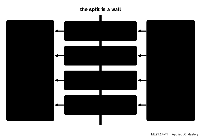
A test error is honest for one reason: the test examples had no influence on the model. A split is a wall. On one side you fit and choose as much as you like. On the other sits the test set, standing in for all the data the model will meet later.
Leakage is anything that gets through the wall. The model, or the person building it, learns something from the test examples, the test error comes out too low, and the surprise arrives later, in use.
ML01.2.4-F1
The split is a wall, and these are the four usual ways through it.
Leaks are quiet. A bug usually makes results worse, and you go looking for it. A leak makes results better, and nobody goes looking.
Build it up
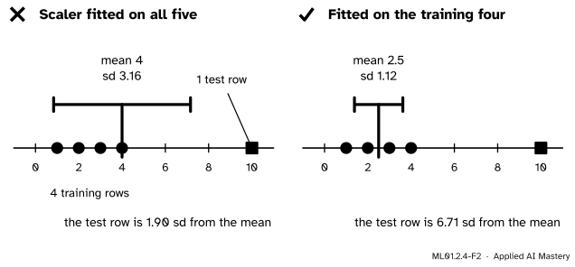
Leak 1. Statistics: scaling before splitting. Many methods work better when each feature is standardised: subtract its mean and divide by its standard deviation (sd), so that values are measured in “sd from the mean”. The mean and the sd are learned from data. From which rows?
Take four training inputs, \(1, 2, 3, 4\), and one test input, \(10\).
ML01.2.4-F2
Wrong beside right. Fitted on all five rows, the scaler’s mean and sd are dragged towards the test row, which then looks ordinary.
Using all five rows, the mean is \(4\) and the sd is \(\sqrt{10} \approx 3.16\), so the test row becomes \({(10 - 4)}/\sqrt{10} \approx 1.90\). Using the four training rows, the mean is \(2.5\) and the sd is \(\sqrt{1.25} \approx 1.12\), so the test row becomes \({(10 - 2.5)}/\sqrt{1.25} \approx 6.71\). Every training input changes too: the input \(1\) is \(-0.95\) in one version and \(-1.34\) in the other. In the first version the training data carry a trace of the test set.
Leak 2. Copies: the same row on both sides. Real datasets contain duplicates: a patient entered twice, a photo saved under two names. If one copy lands in the training set and its twin in the test set, a model that memorises scores perfectly on the twin. The worked example does this by hand.
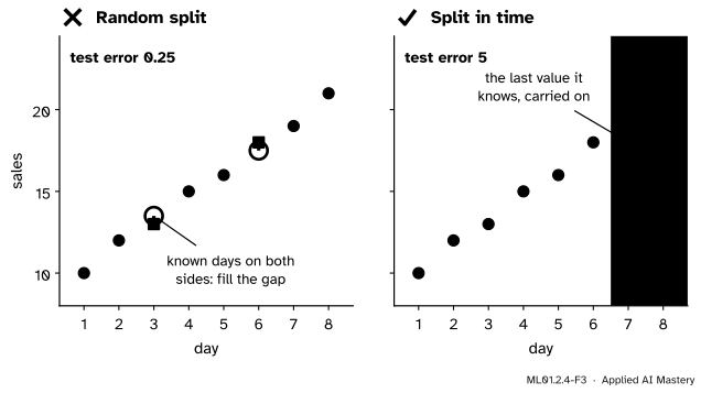
Leak 3. The future: shuffling data that is ordered in time. A shop’s sales on eight days are \(10, 12, 13, 15, 16, 18, 19, 21\). The model answers with the value of the nearest day it knows, or the average if two days are equally near.
ML01.2.4-F3
Wrong beside right. A random split lets the model fill a gap between days it knows. A split in time makes it forecast.
With a random split the test days are \(3\) and \(6\). Each has a known day on either side, so the answers are \({(12 + 15)}/2 = 13.5\) and \({(16 + 19)}/2 = 17.5\), each \(0.5\) off: a test error of \(0.25\). Split in time, the test days are \(7\) and \(8\). The nearest known day is day \(6\), so both answers are \(18\), off by \(1\) and \(3\): a test error of \({(1 + 9)}/2 = 5\), twenty times larger. A forecast is about the future, and a random split tests something easier.
Leak 4. Your choices: peeking at the test set. This leak passes through you. Try twenty models, score each on the test set, and keep the best. The winner was chosen using the test set, which has become a validation set (lesson 2, Result 2).
The formal statement
NoteDefinition: leakage
Leakage is the use, in building or choosing a model, of information that will not be available when the model makes its predictions. Any influence of the test examples on the model is leakage.
One rule prevents all four: split first, and let every step that learns anything learn it from the training set alone. A scaler learns two parameters, a mean and an sd, so it is fitted on the training set and then applied, unchanged, to the other sets.
Result 1: where a duplicate’s twin lands. A dataset of \(N\) rows is shuffled and cut into \(n_{\text{train}}\) training rows and \(n_{\text{test}}\) test rows. Take a test row with exactly one twin elsewhere in the data. Every arrangement is equally likely, so the twin is equally likely to be in any of the other \(N - 1\) places, of which \(n_{\text{train}}\) are training places. So
\[
\begin{aligned}
&\Prob(\text{twin is in the training set}) \\
&\quad = \frac{n_{\text{train}}}{N - 1} .
\end{aligned}
\]
With an 80/20 split this is about \(0.8\). The cure is to split by group: decide what one independent unit is (a patient, a photo), and send all of its rows to the same side of the wall.
Result 2: the best of many guessers. Take a test set of \(n\) yes-or-no questions and a “model” that answers each by tossing a coin. It gets all \(n\) right with probability \((\frac{1}{2})^n = 2^{-n}\), because the tosses are independent, and so fails to be perfect with probability \(1 - 2^{-n}\). Now try \(M\) such models. They are independent, so all of them fail with probability \({(1 - 2^{-n})}^M\), and
\[
\begin{aligned}
&\Prob(\text{at least one of } M \text{ is perfect}) \\
&\quad = 1 - \big(1 - 2^{-n}\big)^M .
\end{aligned}
\]
For \(n = 5\) questions and \(M = 20\) models this is \(1 - (31/32)^{20} \approx 0.47\). Almost half the time, the best of twenty coins is a “perfect” model that knows nothing. Real models are not coins, but the same effect lifts the best of them. A bigger test set weakens it, and a validation set keeps it off the test score.
Frontier note: how much do leaks matter in practice?
Scaling. For a straight line, standardising changes no prediction, and on a few hundred rows the mean and sd barely move without the test rows. The leak grows as the data shrink and as the step learns more. In the scikit-learn guide, on 200 rows of pure noise with 10,000 random features, choosing the “best” features before splitting gives a test accuracy of \(0.76\), when chance is \(0.5\).
Copies. Barz and Denzler (2020) found that 3.3 percent of the test images of CIFAR-10 and 10 percent of those of CIFAR-100, two standard benchmarks of image recognition, have near-duplicates in the training set.
In science. Kapoor and Narayanan (2022) found leakage errors reported in 17 fields that use machine learning, affecting 329 papers.
Worked example
Four examples entered twice, and a lookup table.
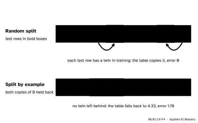
The course’s four points, \((1, 2)\), \((2, 3)\), \((3, 5)\) and \((4, 6)\), are each entered twice by mistake. Call them A, B, C and D. The \(N = 8\) rows are split into 6 training rows and 2 test rows, and the model is the lookup table of lesson 1.
A random split. Suppose the shuffle picks one copy of B and one copy of D for the test set. The training rows are A, A, B, C, C, D, so the table has stored all four inputs. Asked about the test row B, input \(2\), it returns \(3\). Asked about D, input \(4\), it returns \(6\). Both are exactly right: the test error is \(0\).
ML01.2.4-F4
The same eight rows, split two ways.
How likely was that? By Result 1, each test row has its twin in the training set with probability \(n_{\text{train}}/{(N - 1)} = 6/7 \approx 0.86\). Count the splits to check. There are \(\frac{8 \cdot 7}{2} = 28\) ways to choose 2 test rows from 8. In 4 of them the two test rows are twins of each other. In the other 24, each test row has its twin in training and the test error is \(0\). So \(24/28 = 6/7\) of all random splits report a perfect score.
A split by example. Keep the copies together: let both copies of B be the test set. The training rows are A, A, C, C, D, D. The table has no row for the input \(2\), so it falls back to the mean of its stored labels, \({(2 + 2 + 5 + 5 + 6 + 6)}/6 = 26/6 \approx 4.33\). Both test rows have label \(3\), so the test error is \({(4.33 - 3)}^2 = (4/3)^2 \approx 1.78\).
The honest score is \(1.78\). The random split said \(0\).
Code
Leak 1. A scaler from scratch, fitted both ways, and a test for the leak: change the test row and see whether the scaled training inputs move.
import numpy as npx_train, x_test = np.array([1.0, 2, 3, 4]), np.array([10.0])def scale_wrong(train, test): both = np.concatenate([train, test]) # the scaler sees the test rowreturn (train - both.mean()) / both.std(), (test - both.mean()) / both.std()def scale_right(train, test): mean, sd = train.mean(), train.std() # the scaler sees training rows onlyreturn (train - mean) / sd, (test - mean) / sdprint("wrong: test row scaled to", scale_wrong(x_train, x_test)[1].round(2))print("right: test row scaled to", scale_right(x_train, x_test)[1].round(2))other = np.array([100.0]) # a different test rowfor name, scale in [("wrong", scale_wrong), ("right", scale_right)]: moved =not np.allclose(scale(x_train, x_test)[0], scale(x_train, other)[0])print(f"{name}: do the training inputs change when the test row changes? {moved}")
wrong: test row scaled to [1.9]
right: test row scaled to [6.71]
wrong: do the training inputs change when the test row changes? True
right: do the training inputs change when the test row changes? False
Leak 2. The 442 patients of the diabetes dataset, each entered twice, with a lookup table that recognises a stored patient, and the line on body mass index for comparison.
from sklearn.datasets import load_diabetesdata = load_diabetes(scaled=False)bmi, progression = data.data[:, 2], data.targetn =len(bmi) # 442 patientspatient = np.concatenate([np.arange(n), np.arange(n)]) # every patient entered twice: 884 rowsx2, y2 = np.concatenate([bmi, bmi]), np.concatenate([progression, progression])def mse(y_hat, y):return np.mean((y_hat - y) **2)def split(n, n_test, seed): order = np.random.default_rng(seed).permutation(n)return order[:n - n_test], order[n - n_test:]def score(train, test):"""Share of test rows with a twin in training, then the test error of the lookup table and of the line.""" table =dict(zip(patient[train], y2[train])) stored = np.array([table.get(p, y2[train].mean()) for p in patient[test]]) w, b = np.polyfit(x2[train], y2[train], deg=1)return (np.isin(patient[test], patient[train]).mean(), mse(stored, y2[test]), mse(w * x2[test] + b, y2[test]))rows_train, rows_test = split(884, 177, seed=0) # wrong: shuffle the rowswrong = score(rows_train, rows_test)keep, hold = split(n, 89, seed=0) # right: shuffle the patientsright = score(np.flatnonzero(np.isin(patient, keep)), np.flatnonzero(np.isin(patient, hold)))for name, (twins, table_error, line_error) in [("rows", wrong), ("patients", right)]:print(f"split by {name:9} twins in training {twins:4.0%} lookup table {table_error:5.0f} line {line_error:5.0f}")
split by rows      twins in training  77%   lookup table  1652   line  3962
split by patients  twins in training   0%   lookup table  4969   line  4459
Split by rows, 77 percent of the test rows have a twin in training (Result 1 predicts \(707/883 \approx 80\) percent), and the lookup table scores \(1{,}652\) against the line’s \(3{,}962\). Split by patient, it scores \(4{,}969\) against \(4{,}459\). The leak reversed the ranking.
Leak 3. Two hundred days of made-up sales, each the day before plus a random change.
def nearest_day(days_train, values_train, days_query):"""Answer with the stored value of the nearest training day (the mean if two are equally near).""" answers = []for day in days_query: distance = np.abs(days_train - day) answers.append(values_train[distance == distance.min()].mean())return np.array(answers)days8, sales8 = np.arange(1, 9), np.array([10.0, 12, 13, 15, 16, 18, 19, 21])for name, test in [("random split, test days 3 and 6", [2, 5]), ("split in time, test days 7 and 8", [6, 7])]: train = np.setdiff1d(np.arange(8), test)print(f"8 days, {name}: {mse(nearest_day(days8[train], sales8[train], days8[test]), sales8[test]):.2f}")rng = np.random.default_rng(0)days, sales = np.arange(200), 100+ np.cumsum(rng.normal(0.5, 2.0, size=200))train, test = split(200, 40, seed=0)shuffled = mse(nearest_day(days[train], sales[train], days[test]), sales[test])in_time = mse(nearest_day(days[:160], sales[:160], days[160:]), sales[160:])print(f"200 days, random split: {shuffled:.1f} split in time: {in_time:.1f}")
8 days, random split, test days 3 and 6: 0.25
8 days, split in time, test days 7 and 8: 5.00
200 days, random split: 2.5    split in time: 228.7
The random split reports \(2.5\). Forecasting the last 40 days from the first 160 gives \(228.7\), about ninety times worse.
Leak 4. The best of \(M\) coin-tossing models on 50 test questions. Then the same mistake on the diabetes data: keep the table (1 to 60 bins) with the lowest test error, and score it again on 100 patients locked away from the start.
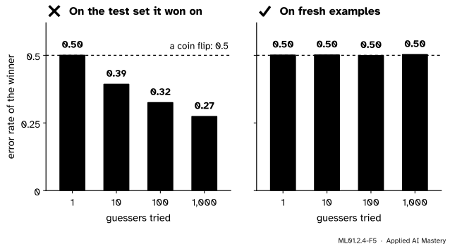
print(f"chance that one of 20 coins is perfect on 5 questions: {1- (31/32) **20:.2f}")rng = np.random.default_rng(0)best_of = {}for count in [1, 10, 100, 1000]: wrong_share = rng.integers(0, 2, size=(2000, count, 50)).mean(axis=2) # error rate of every model fresh = rng.integers(0, 2, size=(2000, 50)).mean() # the winner on new questions best_of[count] = (wrong_share.min(axis=1).mean(), fresh)print(f"best of {count:4d}: error rate {best_of[count][0]:.2f} on the test set, {fresh:.2f} on fresh questions")tenths = np.round(bmi *10).astype(int)def table_errors(bins, train, parts): keys = (tenths -180) * bins //250 counts = np.bincount(keys[train], minlength=bins) sums = np.bincount(keys[train], weights=progression[train], minlength=bins) answers = np.full(bins, progression[train].mean()) answers[counts >0] = sums[counts >0] / counts[counts >0]return [mse(answers[keys[part]], progression[part]) for part in parts]peeked, vaulted = [], []for seed inrange(500): order = np.random.default_rng(seed).permutation(n) train, test, vault = order[:242], order[242:342], order[342:] winner =min((table_errors(bins, train, (test, vault)) for bins inrange(1, 61)), key=lambda e: e[0]) peeked.append(winner[0]) vaulted.append(winner[1])print(f"best of 60 tables: test error {np.mean(peeked):.0f}, the same winners in the vault {np.mean(vaulted):.0f}")
chance that one of 20 coins is perfect on 5 questions: 0.47
best of    1: error rate 0.50 on the test set, 0.50 on fresh questions
best of   10: error rate 0.39 on the test set, 0.50 on fresh questions
best of  100: error rate 0.32 on the test set, 0.50 on fresh questions
best of 1000: error rate 0.27 on the test set, 0.50 on fresh questions
best of 60 tables: test error 3889, the same winners in the vault 4201
The best of 1,000 coins has an error rate of \(0.27\) on the test set that picked it and \(0.50\) elsewhere. On the real data the winning table’s test error averages \(3{,}889\), and on the locked-away patients \(4{,}201\).
The library has a tool for each of the first three leaks.
from sklearn.model_selection import GroupShuffleSplit, train_test_splitfrom sklearn.preprocessing import StandardScalerscaler = StandardScaler().fit(x_train.reshape(-1, 1)) # leak 1: fit on the training rows onlyprint(f"scaler: mean {scaler.mean_[0]}, sd {scaler.scale_[0]:.2f}, test row {scaler.transform([[10.0]])[0, 0]:.2f}")groups = GroupShuffleSplit(n_splits=1, test_size=89, random_state=0) # leak 2: 89 whole patients held outrows_train, rows_test =next(groups.split(x2, y2, groups=patient))print("test rows:", len(rows_test), " patients on both sides:", len(set(patient[rows_train]) &set(patient[rows_test])))past, future = train_test_split(days, test_size=40, shuffle=False) # leak 3: no shuffle, the test set is the endprint("last training day:", past.max(), " first test day:", future.min())
scaler: mean 2.5, sd 1.12, test row 6.71
test rows: 178   patients on both sides: 0
last training day: 159   first test day: 160
For leak 4 the tool is the routine of lesson 2: choose on a validation set, and open the test set once.
Explore
This module’s interactive, the split explorer, is in lesson 3. Try leak 4 there: press Reshuffle until the test error comes out low, and notice that you chose that split by its test score.
Pitfalls
ML01.2.4-F5
Wrong beside right, for leak 4. Every model here is a coin. On the test set that chose it, the best of 1,000 looks skilled. On fresh examples it is a coin again.
“I never trained on the test set. I only used it to pick my best model.”
Picking is a kind of training, done by you. The best of several test scores is partly luck, and the more models you try, the more luck there is to find: \(0.39\), \(0.32\), \(0.27\) in the figure.
“Scaling does not use the labels, so it cannot leak.”
It uses the test inputs. Any number computed from the test rows and then used by the model is a leak, even a mean. On a large dataset the effect of standardising is small, and that is how the habit forms. The same habit with a stronger step can make pure noise look predictable.
“If something had leaked, the results would look strange.”
They look excellent: a leak pushes the test error down. Treat a surprisingly good score as you would a surprisingly bad one, as a reason to check the split.
Check yourself
Recall
1. What is leakage?
Show answer
The use, in building or choosing a model, of information that will not be available when it predicts.
2. Which rows should a scaler’s mean and standard deviation be computed from?
Show answer
The training rows only. The same mean and sd are then applied to the other rows.
3. A dataset contains duplicated rows. How should it be split?
Show answer
By group: all the copies of an example go to the same side.
4. How should data that is ordered in time be split, and why?
Show answer
In time: train on the earlier part and test on the later. In use the model predicts the future, and a random split only tests filling gaps.
5. Why does the best of many models, chosen by test score, look better than it is?
Show answer
Each test score is part skill and part luck, and choosing the best selects for luck as well.
Exercises
1.★ The training inputs are \(2, 4, 6\) and the one test input is \(20\). Standardise the test input with a scaler fitted on all four values, and then with one fitted on the three training values.
Show solution
All four. The mean is \({(2 + 4 + 6 + 20)}/4 = 8\). The squared distances from it are \(36, 16, 4, 144\), with mean \(50\), so the sd is \(\sqrt{50} \approx 7.07\). The test input becomes \({(20 - 8)}/\sqrt{50} \approx 1.70\).
Training three. The mean is \(4\). The squared distances are \(4, 0, 4\), with mean \(8/3\), so the sd is \(\sqrt{8/3} \approx 1.63\). The test input becomes \({(20 - 4)}/\sqrt{8/3} \approx 9.80\).
2.★★ A test set has \(n = 10\) yes-or-no questions. You try \(M = 100\) models that are, in truth, coin tosses. What is the chance that at least one is perfect? How large must \(n\) be for that chance to fall below 1 in 1,000 with the same \(M\)?
When \(M \cdot 2^{-n}\) is small, \({(1 - 2^{-n})}^M\) is close to \(1 - M \cdot 2^{-n}\), so the chance is close to \(M \cdot 2^{-n}\). We need \(100 \cdot 2^{-n} < 0.001\), so \(2^n > 100{,}000\). Since \(2^{16} = 65{,}536\) and \(2^{17} = 131{,}072\), we need \(n \ge 17\). Check: for \(n = 17\) the exact value is \(1 - {(1 - 2^{-17})}^{100} \approx 0.00076\).
3.★★★ A series rises by exactly \(d\) each day: \(v_t = a + d\,t\). The last \(H\) days are held out, and the model is the nearest-day model of this lesson. Show that the test error is \(d^2 {(H + 1)}{(2H + 1)}/6\), and evaluate it for \(d = 0.5\) and \(H = 40\).
Show solution
Let \(T\) be the last training day. For the test day \(T + h\), the nearest known day is \(T\), so the answer is \(v_T\) and the error is \(v_T - v_{T + h} = -h\,d\). The test error is the mean of the squares over \(h = 1, \dots, H\):
using the formula for the sum of the first \(H\) squares. For \(d = 0.5\) and \(H = 40\) this is \(0.25 \cdot 41 \cdot 81 / 6 \approx 138\). The simulated series in the code has this trend plus a random step each day, and its measured error, \(229\), is larger still.
Summary card
A test error is honest only if nothing about the test set reached the model. Split first, and learn everything from the training side.
ML01.2.4-F1
Four ways through the wall.
Statistics. Fit a scaler on the training rows only. Five rows, by hand: \(1.90\) sd (wrong) against \(6.71\) sd (right).
Copies. A test row’s twin is in training with probability \(n_{\text{train}}/{(N - 1)}\). Split by group.
The future. For data ordered in time, test on the end. Eight days: error \(0.25\) (random) against \(5\) (in time).
Your choices. One of \(M\) coins is perfect on \(n\) questions with probability \(1 - {(1 - 2^{-n})}^M\). Choose on validation data.
Sources and next steps
Sources. Each was opened and checked against this lesson on 12 November 2026.
scikit-learn developers, Common pitfalls and recommended practices, User Guide, Section 12.2, Data leakage (version 1.9.1). Defines data leakage as using information that would not be available at prediction time, states that test data should never be used to make choices about the model, and gives the feature-selection example on random data (accuracy 0.76 the wrong way, 0.5 the right way).
scikit-learn developers, Cross-validation: evaluating estimator performance, User Guide (version 1.9.1). Section 3.1.2.4 covers grouped data, with patients measured several times as its example. Section 3.1.2.6 states that time-series models should be evaluated on “future” observations.
Björn Barz and Joachim Denzler, Do We Train on Test Data? Purging CIFAR of Near-Duplicates, Journal of Imaging 6(6):41, 2020. The abstract reports that 3.3% and 10% of the test images of CIFAR-10 and CIFAR-100 have duplicates in the training set.
Next. Module ML01.3, k-nearest neighbours, builds a model that stores its training set and still generalises, and chooses its one hyperparameter on a validation set.