Training error flatters a model, and a test error is only an estimate. Measure both on real data, watch the gap between them open as a model gets more flexible, and learn why a test score moves when the split changes and how more test examples steady it.
Define the generalisation gap and compute it from a training error and a test error.
Describe, from measurements on real data, how the gap changes as a model is made more flexible.
Explain why a test error changes when the split is reshuffled, and measure by how much.
Compute the standard error of a test error and say how it shrinks as the test set grows.
Judge whether the difference between two test errors is large enough to trust.
In review. The maths and code on this page are checked by automated tests on every change, but an independent reader has not signed it off yet. Spot a mistake or a confusing step? Tell us.
The question
Lesson 2 ended with a report: on 89 test patients, the line’s error was \(4{,}418\), against \(3{,}728\) on its own training patients. How much better does a model look on the data it was fitted to? And would 89 different patients have given the same number?
From the last lesson
1. Which set is used to choose between models, and which to report on the winner?
Show answer
The validation set chooses. The test set reports, once, and decides nothing.
2. What does a seed do, and why record it?
Show answer
It fixes the shuffle: the same seed gives the same split every time, so the results can be reproduced.
Intuition
Every fitted model has two errors: one on the examples it was fitted to, and one on examples held back. The generalisation gap is the second minus the first:
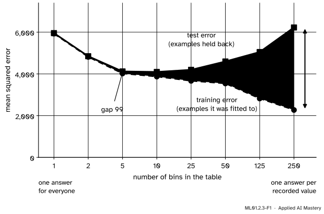
The picture measures the gap on real data, for the tables of lesson 2, from 1 bin to 250. The data are the 442 patients of scikit-learn’s diabetes dataset, the input is the body mass index, and each point is an average over 1,000 splits.
ML01.2.3-F1
With few bins the two errors are nearly equal. As bins are added the training error keeps falling, the test error turns back up, and the shaded gap opens.
Two things are in this picture. One is the gap: small for a simple model, large for a flexible one. The other hides in the words “average over 1,000 splits”: a single split gives one noisy copy of each point. A test error is a measurement, with a give-or-take.
Build it up
Step 1. One split, two numbers for each model. This lesson needs only two sets, so lesson 2’s validation patients rejoin the training set: 353 patients to train on, the same 89 to test on. The models are the line and the tables with 1, 5, 25 and 250 bins.
Model
Training error
Test error
Gap
Line
\(3{,}756\)
\(4{,}459\)
\(703\)
1 bin
\(6{,}172\)
\(4{,}969\)
\(-1{,}204\)
5 bins
\(3{,}986\)
\(4{,}239\)
\(253\)
25 bins
\(3{,}600\)
\(4{,}392\)
\(792\)
250 bins
\(2{,}228\)
\(5{,}990\)
\(3{,}762\)
(Here and in Step 2, gaps are computed before rounding, so some differ by \(1\).)
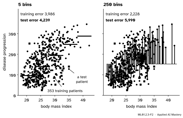
ML01.2.3-F2
The same split, two tables. With 5 bins the model is a staircase through the cloud. With 250 it jumps to almost every training patient.
The lookup table, 250 bins, has by far the largest gap, as in lesson 1. But the one-bin table, whose single parameter is the mean, scores \(1{,}204\)better on patients it has never met. No model is that modest.
Step 2. Reshuffle. Split the 442 patients again with a different seed, 1,000 times, and average.
Model
Mean training error
Mean test error
Mean gap
Line
\(3{,}888\)
\(3{,}922\)
\(34\)
1 bin
\(5{,}928\)
\(5{,}954\)
\(26\)
5 bins
\(4{,}020\)
\(4{,}118\)
\(99\)
25 bins
\(3{,}666\)
\(4{,}196\)
\(529\)
250 bins
\(2{,}272\)
\(6{,}224\)
\(3{,}953\)
Models with one or two parameters have a gap of about 30, under one percent of their error. The gap grows with flexibility and reaches almost \(4{,}000\) for the lookup table. The \(-1{,}204\) of Step 1 was luck: those 89 test patients happened to be less spread out than the rest.
Step 3. In practice you get one split. How far can one test error stray? Over the 1,000 splits the line’s test error ran from \(2{,}691\) to \(5{,}209\), with a standard deviation of \(457\). The \(4{,}459\) of Step 1 was a high draw: higher than 87 percent of the others.
Step 4. More test examples, less straying. Repeat with test sets of different sizes.
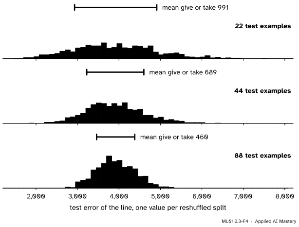
ML01.2.3-F4
The line’s test error over 1,000 reshuffled splits. The centre does not move. The width does: four times as many test examples roughly halve it, from \(991\) to \(460\).
The formal statement
NoteDefinition: generalisation gap
For a model \(f\) fitted on a training set and scored on a test set,
On average the gap is not negative, because the parameters were chosen to make the training error small. In a single split it can have either sign.
Result: the standard error of a test error. Write \(\ell_j = {(f(x'_j) - y'_j)}^2\) for the squared miss on test example \(j\): the loss on that one example. The test error is the mean of these:
Treat the test examples as independent draws from the source of the data. Then each \(\ell_j\) is a draw from one distribution of losses, with some mean \(\mu\) and standard deviation \(s\). The mean \(\mu\) is the generalisation error of lesson 1, the number we are after.
Spread is easiest to track through the variance, the square of the standard deviation. Two facts, proved in the block below, suffice.
Fact A. The variance of a sum of independent quantities is the sum of their variances.
Fact B. Multiplying a quantity by a constant \(c\) multiplies its variance by \(c^2\).
By Fact A, the sum \(\ell_1 + \dots + \ell_{n_{\text{test}}}\) has variance \(n_{\text{test}}\, s^2\). The test error is that sum times \(1/n_{\text{test}}\), so by Fact B its variance is
Take the square root to return to a standard deviation:
\[
\text{standard error of } L_{\text{test}} \;=\; \frac{s}{\sqrt{n_{\text{test}}}} .
\]
The standard error is the typical distance between the test error you measured and the generalisation error you wanted. Three things follow.
To halve it you need four times as many test examples.
Only the number of test examples appears, not their share of the dataset.
You can estimate it from one split: take \(s\) to be the standard deviation of the losses on your own test set.
Go deeper: the two facts about variance
The variance of a quantity \(X\) with mean \(\mu_X\) is its average squared distance from the mean, \(\E[{(X - \mu_X)}^2]\).
Fact B. The mean of \(cX\) is \(c\mu_X\), so its variance is \(\E[{(cX - c\mu_X)}^2] = c^2\, \E[{(X - \mu_X)}^2]\), which is \(c^2\) times the variance of \(X\).
Fact A. Let \(X\) and \(Y\) have means \(\mu_X\) and \(\mu_Y\). Their sum has mean \(\mu_X + \mu_Y\), so its variance is
The outer terms are the two variances. When \(X\) and \(Y\) are independent, the average of a product is the product of the averages, so the middle term is \(2\,\E[X - \mu_X]\,\E[Y - \mu_Y] = 2 \cdot 0 \cdot 0 = 0\). Adding one quantity at a time covers a sum of any length.
Go deeper: a formula for the gap of a table: twice the noise, divided by the bin's head count
Take one bin of a table, holding \(k\) training examples whose labels are independent draws with mean \(\mu\) and variance \(\sigma^2\): inside the bin there is no pattern, only noise. The stored answer is their mean, \(\bar{y}\), which has mean \(\mu\) and, by Facts A and B, variance \(\sigma^2/k\).
Test error. A new example in the bin has a label \(y'\), independent of \(\bar{y}\). Write \(y' - \bar{y} = {(y' - \mu)} - {(\bar{y} - \mu)}\). The brackets are independent and have mean \(0\), so by Fact A (and Fact B with \(c = -1\)) the expected squared miss is
Training error. Write \(y_i - \mu = {(y_i - \bar{y})} + {(\bar{y} - \mu)}\), square, and add over the \(k\) stored examples. The cross term carries the factor \(\sum_i {(y_i - \bar{y})} = 0\), so
Averaging both sides gives \(k\sigma^2 = \E\big[\sum_i {(y_i - \bar{y})}^2\big] + k \cdot \sigma^2/k\), so the expected training error in the bin is \({(k - 1)}\sigma^2 / k = \sigma^2 {(1 - 1/k)}\).
A bin that holds one example memorises it: training error \(0\), test error \(2\sigma^2\). A bin that averages many has almost no gap. Flexibility opens the gap by leaving fewer examples behind each answer.
Worked example
Find the gap and the standard error for both models of lesson 1.
The four new examples of lesson 1 are a test set of size \(4\). From that lesson, the line has \(L_{\text{train}} = 0.05\) and \(L_{\text{test}} = 0.09\), and the lookup table has \(0\) and \(2.75\).
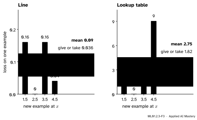
Standard error for the line. Its four losses are \(0.16\), \(0\), \(0.16\) and \(0.04\), with mean \(0.09\). Their distances from the mean are \(0.07\), \(-0.09\), \(0.07\) and \(-0.05\), and the squares of those are \(0.0049\), \(0.0081\), \(0.0049\) and \(0.0025\). So
Standard error for the lookup table. Its losses are \(1\), \(0\), \(1\) and \(9\), with mean \(2.75\). The distances from the mean are \(-1.75\), \(-2.75\), \(-1.75\) and \(6.25\), and their squares add up to \(3.0625 + 7.5625 + 3.0625 + 39.0625 = 52.75\). So
A test error is the mean of a few losses. The yellow band is one standard error either side.
So the reports are: line, \(0.09\) give or take \(0.04\); lookup table, \(2.75\) give or take \(1.82\). The low end of the table’s range, about \(0.93\), is above the high end of the line’s, about \(0.13\). That favours the line, though four examples make a rough band: one loss of \(9\) supplies most of the table’s error.
On the real data. For the line of Step 1, the 89 test losses have mean \(4{,}459\) and \(s = 5{,}110\), so the standard error is \(5{,}110/\sqrt{89} \approx 542\). The 5-bin table scored \(4{,}239\) on the same patients, \(220\) lower. The yardstick for a difference is the standard error of the 89 differences, the table’s loss minus the line’s for each patient. It is \(184\). A lead of \(1.2\) standard errors often arises by chance, so this test set cannot rank the two.
(Statisticians divide by \(n - 1\), not \(n\), in \(s\): half a percent more with 89 examples.)
Code
The line and lesson 2’s table from scratch. The table now uses arrays, to be fitted thousands of times.
import numpy as npfrom sklearn.datasets import load_diabetesdata = load_diabetes(scaled=False) # 442 patients (see lesson 2)bmi, progression = data.data[:, 2], data.targettenths = np.round(bmi *10).astype(int) # BMI in tenths, so that the bins are exactn =len(bmi)def mse(y_hat, y):return np.mean((y_hat - y) **2)def split(n, n_test, seed):"""Shuffle the example numbers with a seed. The last n_test are the test set.""" order = np.random.default_rng(seed).permutation(n)return order[:n - n_test], order[n - n_test:]def errors(model, train, test):"""Training error and test error of the line, or of a table with `model` bins."""if model =="line": w, b = np.polyfit(bmi[train], progression[train], deg=1) predict =lambda rows: w * bmi[rows] + belse: keys = (tenths -180) * model //250# the bin of every patient counts = np.bincount(keys[train], minlength=model) sums = np.bincount(keys[train], weights=progression[train], minlength=model) answers = np.full(model, progression[train].mean()) # an empty bin: the training mean answers[counts >0] = sums[counts >0] / counts[counts >0] # any other bin: its own mean predict =lambda rows: answers[keys[rows]]return mse(predict(train), progression[train]), mse(predict(test), progression[test])MODELS = ["line", 1, 5, 25, 250]train, test = split(n, n_test=89, seed=0) # the same 89 test patients as in lesson 2for model in MODELS: training, testing = errors(model, train, test)print(f"{str(model):>5} training {training:5.0f} test {testing:5.0f} gap {testing - training:6.0f}")
 line   training  3756   test  4459   gap    703
    1   training  6172   test  4969   gap  -1204
    5   training  3986   test  4239   gap    253
   25   training  3600   test  4392   gap    792
  250   training  2228   test  5990   gap   3762
Now 1,000 splits, each with its own seed.
runs = {model: np.array([errors(model, *split(n, 89, seed)) for seed inrange(1000)]) for model in MODELS}for model, r in runs.items():print(f"{str(model):>5} mean training {r[:, 0].mean():5.0f} mean test {r[:, 1].mean():5.0f} "f"mean gap {(r[:, 1] - r[:, 0]).mean():5.0f}")line_tests = runs["line"][:, 1]print(f"line, test error: lowest {line_tests.min():.0f}, highest {line_tests.max():.0f}, "f"standard deviation {line_tests.std():.0f}")print(f"splits where the line's test error is below its training error: "f"{np.mean(runs['line'][:, 1] < runs['line'][:, 0]):.0%}")print(f"splits where the 5-bin table beats the line on the test set: "f"{np.mean(runs[5][:, 1] < line_tests):.0%}")
 line   mean training  3888   mean test  3922   mean gap    34
    1   mean training  5928   mean test  5954   mean gap    26
    5   mean training  4020   mean test  4118   mean gap    99
   25   mean training  3666   mean test  4196   mean gap   529
  250   mean training  2272   mean test  6224   mean gap  3953
line, test error: lowest 2691, highest 5209, standard deviation 457
splits where the line's test error is below its training error: 50%
splits where the 5-bin table beats the line on the test set: 14%
Half the time the line’s test error fell below its training error, and the 5-bin table, worse on average, beat it in 14 percent of the splits.
Next, the standard error from one split, and the spread for three test-set sizes.
w, b = np.polyfit(bmi[train], progression[train], deg=1)losses = (w * bmi[test] + b - progression[test]) **2# the loss on each test patientprint(f"seed 0: test error {losses.mean():.0f}, s = {losses.std():.0f}, "f"standard error = {losses.std() / np.sqrt(89):.0f}")keys = (tenths -180) *5//250# the 5-bin table on the same splitanswers = np.array([progression[train][keys[train] == k].mean() for k inrange(5)])differences = (answers[keys[test]] - progression[test]) **2- losses # table's loss minus line'sprint(f"table minus line: mean {differences.mean():.0f}, s = {differences.std():.0f}, "f"standard error = {differences.std() / np.sqrt(89):.0f}")w_all, b_all = np.polyfit(bmi, progression, deg=1)s_all = ((w_all * bmi + b_all - progression) **2).std() # s measured on all 442 patientsprint(f"s over all patients = {s_all:.0f}")for n_test in [22, 44, 88]: tests = np.array([errors("line", *split(n, n_test, seed))[1] for seed inrange(1000)])print(f"{n_test:3d} test patients spread over 1,000 splits {tests.std():4.0f} "f"s / sqrt(n_test) = {s_all / np.sqrt(n_test):4.0f}")
seed 0: test error 4459, s = 5110, standard error = 542
table minus line: mean -220, s = 1738, standard error = 184
s over all patients = 4689
 22 test patients   spread over 1,000 splits  991   s / sqrt(n_test) = 1000
 44 test patients   spread over 1,000 splits  689   s / sqrt(n_test) =  707
 88 test patients   spread over 1,000 splits  460   s / sqrt(n_test) =  500
The formula predicts \(1{,}000\), \(707\) and \(500\). The measured \(991\), \(689\) and \(460\) fall a little short, most for the largest test set. The formula is for examples drawn afresh, but a reshuffle draws them without repeats from a fixed pool of \(N = 442\) patients, and a sample that uses up much of its pool strays less. Multiplying by
\[
\sqrt{\frac{N - n_{\text{test}}}{N - 1}}
\]
allows for this: \(976\), \(672\) and \(448\). Reshuffling slightly understates the give-or-take of a fresh test set.
The library’s tool for repeated random splits is ShuffleSplit. It hands out the row numbers of each split.
from sklearn.linear_model import LinearRegressionfrom sklearn.metrics import mean_squared_errorfrom sklearn.model_selection import ShuffleSplitX = bmi.reshape(-1, 1)library = []for rows_train, rows_test in ShuffleSplit(n_splits=200, test_size=89, random_state=0).split(X): model = LinearRegression().fit(X[rows_train], progression[rows_train]) library.append(mean_squared_error(progression[rows_test], model.predict(X[rows_test])))print(f"ShuffleSplit, 200 splits: mean test error {np.mean(library):.0f}, spread {np.std(library):.0f}")
ShuffleSplit, 200 splits: mean test error 3907, spread 419
The same picture.
Explore
ML01.2-X1
Split explorer
Thirty made-up points, a curve plus noise, are split into a training set and a test set. Slide the number of bins up: the training error falls while the test error turns back up. Press Reshuffle 20 times to see how far the test error moves. Then, at one bin, enlarge the test set and watch the marks bunch together.
Pitfalls
ML01.2.3-F5
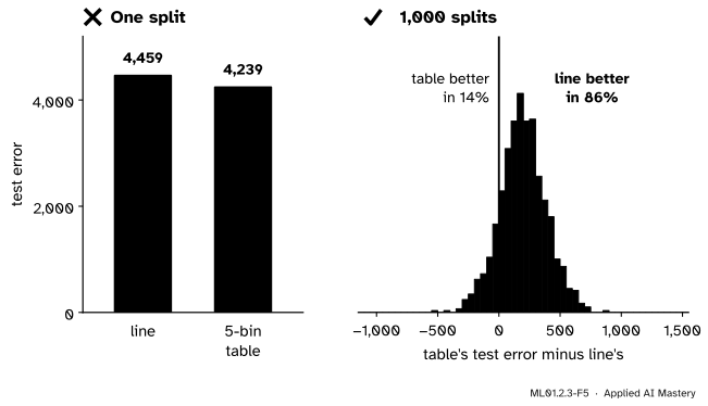
Wrong beside right. On one split the 5-bin table has the lower test error. Over 1,000 splits the line wins 86 percent of the time.
“Model A scored lower than model B on the test set, so A is better.”
Only if the difference is large beside its own give-or-take. In Step 1 the table won by \(220\), and the standard error of that difference is \(184\). Compute it, or repeat the split.
“Test error is always higher than training error.”
On average, yes. In a single split, no: for the line it was lower in half of the 1,000 splits.
“A small gap means a good model.”
The one-bin table has the smallest gap of all, \(26\), and a test error of \(5{,}954\), far worse than the line’s. A small gap says the training error can be trusted, not that it is low.
Check yourself
Recall
1. Define the generalisation gap.
Show answer
The test error of a fitted model minus its training error.
2. On the diabetes data, how does the average gap change as the table is given more bins?
Show answer
It grows: \(26\) with 1 bin, \(99\) with 5, \(529\) with 25 and \(3{,}953\) with 250.
3. The same kind of model is fitted on reshuffled splits and its test error changes each time. Why?
Show answer
It is the mean of the losses on one sample of test examples, and a different sample has a different mean.
4. What is the standard error of a test error, and what happens to it when the test set is made four times larger?
Show answer
It is \(s/\sqrt{n_{\text{test}}}\), where \(s\) is the standard deviation of the per-example losses. Four times as many test examples halve it.
5. A model has a very small gap. Is it a good model?
Show answer
Not necessarily. A small gap means its training error is a fair guide to its test error. Both may be high, as for the one-bin table.
Exercises
1.★ A model has training error \(1{,}200\). On a test set of \(400\) examples its test error is \(1{,}500\), and the standard deviation of the 400 losses is \(2{,}000\). Find the gap and the standard error of the test error.
Show solution
The gap is \(1{,}500 - 1{,}200 = 300\). The standard error is \(s/\sqrt{n_{\text{test}}} = 2{,}000/\sqrt{400} = 2{,}000/20 = 100\).
2.★★ A classifier is wrong on 10 of 100 test examples. Score each example \(1\) if the prediction is wrong and \(0\) if it is right, so that the test error is the error rate, \(p = 0.1\). Show that the standard deviation of these scores is \(\sqrt{p(1 - p)}\), find the standard error, and find how many test examples would bring it down to \(0.01\).
Show solution
The mean of the scores is \(p\). A share \(p\) of them equal \(1\), at distance \(1 - p\) from the mean, and a share \(1 - p\) equal \(0\), at distance \(p\). So the mean squared distance is
and \(s = \sqrt{p(1 - p)} = \sqrt{0.1 \cdot 0.9} = 0.3\). The standard error is \(0.3/\sqrt{100} = 0.03\): the error rate is “10 percent, give or take 3 points”.
For a standard error of \(0.01\) we need \(0.3/\sqrt{n_{\text{test}}} = 0.01\), so \(\sqrt{n_{\text{test}}} = 30\) and \(n_{\text{test}} = 900\).
3.★★★ By the second deeper block, a bin holding \(k\) training examples has an expected gap of \(2\sigma^2/k\). Predict the average gap of the one-bin table on the diabetes data, where \(k = 353\) and the variance of the label is about \(5{,}930\). How many training patients would bring it below \(10\)?
Show solution
A model that answers with the mean leaves the whole variance of the label as noise, so \(\sigma^2 \approx 5{,}930\) and the predicted gap is \(2 \cdot 5{,}930 / 353 \approx 34\). The measured \(26\) is within the noise: one split’s gap has a standard deviation of about \(730\), so a mean over 1,000 splits has a standard error of about \(730/\sqrt{1{,}000} \approx 23\).
For a gap below \(10\) we need \(2 \cdot 5{,}930 / k < 10\), so \(k > 1{,}186\) patients.
Summary card
A model looks better on its own training data by the gap, and a test error is a measurement with a give-or-take.
ML01.2.3-F1
The gap opens with flexibility.
Gap.\(\text{gap} = L_{\text{test}} - L_{\text{train}}\). Small for simple models, large for flexible ones. Not negative on average.
Standard error.\(L_{\text{test}}\) is a mean of \(n_{\text{test}}\) losses, so it strays by about \(s/\sqrt{n_{\text{test}}}\). Four times the test set halves that.
Diabetes data, line. Mean training error \(3{,}888\), mean test error \(3{,}922\), gap \(34\). One test set of 89: give or take about \(500\).
Sources and next steps
Sources. Each was opened and checked against this lesson on 12 November 2026.
Ian Goodfellow, Yoshua Bengio and Aaron Courville, Deep Learning, MIT Press, 2016. Section 5.2: the expected test error is at least the expected training error, and the aims are a small training error and a small gap between the two (Figure 5.3 marks the generalisation gap). Section 5.3.1: a small test set implies statistical uncertainty around the estimated test error.
OpenStax, Introductory Statistics 2e, Section 7.1. The standard deviation of a sample mean is that of the original distribution divided by the square root of \(n\): the standard error of the mean.
scikit-learn developers, ShuffleSplit, API reference (version 1.9.1). A random permutation cross-validator that yields indices of repeated training and test splits.
scikit-learn developers, Diabetes dataset, User Guide, Section 9.1.2. 442 patients, ten baseline variables and a measure of disease progression a year later.
Next.ML01.2.4 How splits go wrong is about test errors that are too good to be true, and the four leaks that cause them.