A model that simply stores its training examples scores perfectly on them and fails on anything new. See memorising and generalising side by side, a lookup table against a straight line, and learn why a score on seen data proves nothing.
Tell memorising from generalising, and say which of the two a score on the training data rewards.
Compute by hand the training error and the error on new examples of a lookup table and of a line.
Prove that a lookup table has zero training error on any dataset whose inputs are all different.
Explain why models with the same training error can disagree on every input they have not seen.
In review. The maths and code on this page are checked by automated tests on every change, but an independent reader has not signed it off yet. Spot a mistake or a confusing step? Tell us.
The question
A student gets hold of last year’s exam paper with its answers, learns every answer by heart, and then sits that same paper. Full marks. Has the student learned the subject? Every score you will ever read for a machine learning model is an answer to this question, and the score is only honest if the exam was new.
Intuition
Module ML01.1 ended with a recipe for learning. Pick a model, a family of functions (lesson ML01.1.3). Score every setting of its parameters with a loss, and keep the setting with the lowest loss (lesson ML01.1.4). That recipe has a hole in it. A low loss on the examples we have can be reached in two very different ways.
Memorising. Store the examples, and give back the stored answer when asked.
Generalising. Find the pattern behind the examples, so that the answer is also right for inputs nobody has shown you.
To see the difference, take the course’s four points, \((1, 2)\), \((2, 3)\), \((3, 5)\) and \((4, 6)\), and build two models from them. As lesson ML01.1.3 allows after training, “model” now means the one chosen member of a family. The examples a model is built from are its training set.
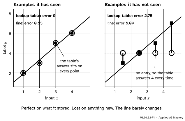
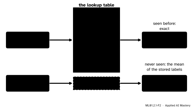
The first model is a lookup table. It stores the four pairs. Asked about an input it has stored, it returns the stored label. Asked about any other input, it has nothing to go on and returns one fixed answer: the average of its stored labels, \(4\).
The second model is the straight line \(\hat{y} = 1.4x + 0.5\). It is the line that fits the four points best (module ML01.4 finds it). It has only two parameters, so it cannot store four answers and has to summarise them.
ML01.2.1-F1
Two models built from the same four examples, scored by mean squared error. Left: on those four, the lookup table is perfect. Right: on four new examples, its error jumps from \(0\) to \(2.75\), while the line’s moves from \(0.05\) to \(0.09\).
Judged on the examples it has seen, the lookup table is the better model. Judged on four examples that neither model has met, it is about thirty times worse than the line.
The first score was not wrong. It answered the wrong question: “can you repeat what you were shown?” A table of stored answers always can. The question that matters is “what will you say about something new?”
Build it up
Step 1. What a lookup table is. It has no formula. Its only contents are the rows it was given.
ML01.2.1-F2
The parts of a lookup table: a stored row for a query it has seen, and a fallback for one it has not.
Step 2. Score it on what it stored. Ask the table about \(x = 1, 2, 3, 4\). Each query finds its row, so each answer equals its label and each miss, answer minus label, is zero. Swap the four labels for any other numbers and the loss is still a perfect zero.
Step 3. Score it on something new. Now ask about \(x = 1.5, 2.5, 3.5, 4.5\). No query finds a row. The table answers \(4\) four times, and it is badly wrong for the largest input.
Step 4. Do the same for the line. The line cannot pass through all four training points, so its loss on them is a little above zero. In exchange it has an answer for every input, one that follows the trend. Its loss on the new examples is nearly the same as on the old.
Step 5. Name the two scores. The loss on the examples a model was built from is its training error. The same loss on examples kept away from the building is its test error, and those examples are a test set. A model generalises when its test error is low. The table memorises: training error low, test error high. The line generalises: both low.
The rule of this module, in its first form: never judge a model by the examples it was built from.
The formal statement
NoteDefinition: training error and test error
A fitted model \(f\) turns an input \(x\) into an answer \(\hat{y} = f(x)\), its prediction. The loss is the mean squared error. For the \(n\) training examples \((x_1, y_1), \dots, (x_n, y_n)\) and for \(m\) other examples \((x'_1, y'_1), \dots, (x'_m, y'_m)\) that were not used to build \(f\),
The two formulas are the same. Only the examples differ.
Result 1: a lookup table has training error zero, whatever the data. Suppose the training inputs \(x_1, \dots, x_n\) are all different. The table stores the pair \((x_i, y_i)\) for every \(i\), so for a training input it returns the stored label: \(f(x_i) = y_i\). Then
Nothing about the labels was used: they could be measurements or random numbers. A score that is perfect for every possible dataset tells you nothing about this one.
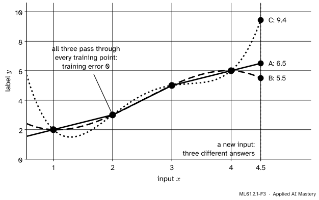
Result 2: training error is blind between the training points. Let \(f\) and \(g\) be two models that agree on the training inputs: \(f(x_i) = g(x_i)\) for every \(i\). Each term of the training error contains the model only through its value at \(x_i\), so
They may give any answers at all for every other input, and the training error cannot see it.
ML01.2.1-F3
Three models with training error exactly \(0\) on the four points. At the new input \(x = 4.5\) they answer \(6.5\), \(5.5\) and \(9.4\). Nothing in the training error says which to trust.
Result 3: what we want, and how to estimate it. The number that matters is the loss on the examples the model will meet in use. Think of those as drawn from the same source as the training examples. The average squared miss over fresh draws \((X, Y)\) from that source is the generalisation error,
Nobody can compute it, because nobody has the whole source. The test error, an average over a held-back sample, is our estimate of it. The training error is not a fair estimate, because the model was chosen to make that very number small.
Go deeper: why the table falls back to the mean, and what happens when an input repeats
If a model must give one answer \(c\) for a set of labels \(y_1, \dots, y_k\), which \(c\) has the lowest mean squared error? Write \(\bar{y}\) for the mean of the labels and split each difference in two: \(c - y_j = {(c - \bar{y})} + {(\bar{y} - y_j)}\). Squaring gives
The second term does not contain \(c\). The first is never negative and is zero only when \(c = \bar{y}\). So the mean is the best single answer, as lesson ML01.1.4 found by completing the square. For the four labels \(2, 3, 5, 6\) the mean is \(4\) and its error is \({(4 + 1 + 1 + 4)}/4 = 2.5\): no constant can do better on the training set.
If an input repeats, say \(x = 2\) twice with labels \(3\) and \(4\), the table can store only one answer for it. The best is their mean, \(3.5\), and the training error is then above zero. That is why Result 1 needs the inputs to be different.
Frontier note: large neural networks can memorise too
Memorising is not only a toy problem. Zhang and co-authors (2017) gave every training image a random label, so that there was no pattern left to learn. Standard image classifiers still fitted the training set, as a lookup table would, and explicit regularisation made little difference. So fitting the training set cannot be what makes these networks do well on new images.
Worked example
Compute the training error and the test error of both models by hand.
The training examples are \((1, 2)\), \((2, 3)\), \((3, 5)\), \((4, 6)\). The four new examples, made up to follow the same rising pattern, are \((1.5, 3)\), \((2.5, 4)\), \((3.5, 5)\) and \((4.5, 7)\).
The lookup table on the training examples. Every answer equals its label, so every squared miss is \(0\) and \(L_{\text{train}} = 0\).
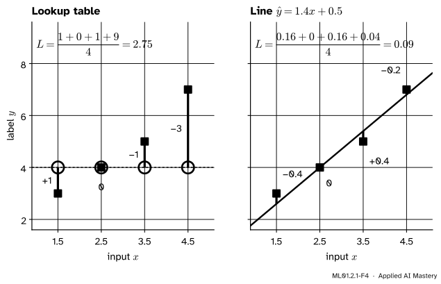
The lookup table on the new examples. None of \(1.5, 2.5, 3.5, 4.5\) is stored, so every answer is the fallback, \({(2 + 3 + 5 + 6)}/4 = 4\).
The line on the training examples. The answers \(1.4x + 0.5\) are \(1.9, 3.3, 4.7, 6.1\). The misses are \(-0.1, 0.3, -0.3, 0.1\) and their squares are \(0.01, 0.09, 0.09, 0.01\), so \(L_{\text{train}} = 0.20/4 = 0.05\).
The line on the new examples. Each answer is \(1.4x + 0.5\).
The two tables as a picture. Each purple bar is one miss on a new example.
Model
Training error
Test error
Lookup table
\(0\)
\(2.75\)
Line
\(0.05\)
\(0.09\)
The first column ranks the lookup table first, the second last, by a factor of \(2.75 / 0.09 \approx 31\). Only the second describes what happens in use.
Code
Both models from scratch. The lookup table is a Python dictionary.
import numpy as npx_train = np.array([1.0, 2.0, 3.0, 4.0]) # the examples both models are built fromy_train = np.array([2.0, 3.0, 5.0, 6.0])x_new = np.array([1.5, 2.5, 3.5, 4.5]) # four examples neither model has seeny_new = np.array([3.0, 4.0, 5.0, 7.0])def mse(y_hat, y):"""Mean squared error: the average of the squared differences."""return np.mean((y_hat - y) **2)table =dict(zip(x_train, y_train)) # the memoriser: input -> stored labelfallback = y_train.mean() # its answer for an input it has never storeddef table_predict(x):return np.array([table.get(xi, fallback) for xi in x])def line_predict(x, w=1.4, b=0.5): # the best-fitting line through the four pointsreturn w * x + bfor name, predict in [("lookup table", table_predict), ("line", line_predict)]:print(f"{name:13} training error {mse(predict(x_train), y_train):.2f} "f"test error {mse(predict(x_new), y_new):.2f}")
lookup table  training error 0.00   test error 2.75
line          training error 0.05   test error 0.09
Result 1 says the table’s perfect score does not depend on the labels. So give both models 1,000 examples whose labels are pure noise, and then 1,000 fresh ones.
rng = np.random.default_rng(0)x_big = np.arange(1000.0) # 1,000 different inputsy_noise = rng.normal(size=1000) # labels drawn at random: there is nothing to learnx_fresh = x_big +0.5# 1,000 new inputs from the same sourcey_fresh = rng.normal(size=1000)noise_table =dict(zip(x_big, y_noise))def noise_table_predict(x):return np.array([noise_table.get(xi, y_noise.mean()) for xi in x])w, b = np.polyfit(x_big, y_noise, deg=1) # the least-squares lineprint(f"lookup table training error {mse(noise_table_predict(x_big), y_noise):.2f} "f"test error {mse(noise_table_predict(x_fresh), y_fresh):.2f}")print(f"line training error {mse(w * x_big + b, y_noise):.2f} "f"test error {mse(w * x_fresh + b, y_fresh):.2f}")
lookup table  training error 0.00   test error 1.05
line          training error 0.95   test error 1.04
The table reports a perfect fit to noise. The line’s training error, close to \(1\), is the honest figure: the variance of the noise, which both models score on fresh examples.
Now the library. scikit-learn’s nearest relative of a lookup table is the 1-nearest-neighbour model of module ML01.3, which stores the training set and answers with the label of the closest stored input.
from sklearn.linear_model import LinearRegressionfrom sklearn.metrics import mean_squared_errorfrom sklearn.neighbors import KNeighborsRegressorX_train, X_new = x_train.reshape(-1, 1), x_new.reshape(-1, 1) # scikit-learn wants a columnline = LinearRegression().fit(X_train, y_train)memoriser = KNeighborsRegressor(n_neighbors=1).fit(X_train, y_train)print(f"line: w = {line.coef_[0]:.2f}, b = {line.intercept_:.2f}, "f"training error {mean_squared_error(y_train, line.predict(X_train)):.2f}, "f"test error {mean_squared_error(y_new, line.predict(X_new)):.2f}")print(f"1-nearest neighbour: training error "f"{mean_squared_error(y_train, memoriser.predict(X_train)):.2f}")
line: w = 1.40, b = 0.50, training error 0.05, test error 0.09
1-nearest neighbour: training error 0.00
The 1-nearest-neighbour model also scores \(0\) on its own training set, for the same reason. That zero is true and useless.
Explore
This module’s interactive, the split explorer, is in lesson 3. It slides a table from one answer for everyone to a full lookup table, and the training and test errors part company.
Pitfalls
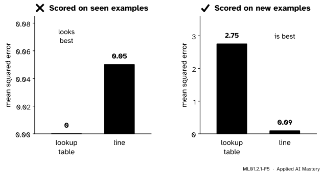
ML01.2.1-F5
Wrong beside right. The two charts rank the same two models in opposite orders. Note the scales: the left one stops at \(0.08\).
“My model gets everything right on the data, so it has learned the pattern.”
If “the data” means the examples it was built from, a lookup table gets everything right too, even when the labels are random. Ask for the score on examples the model has never met.
“The model with the lower training error is the better model.”
Here the training errors are \(0\) and \(0.05\), and the test errors are \(2.75\) and \(0.09\). The order flips.
“So storing the training data is always a mistake.”
Storing is fine. The 1-nearest-neighbour model of module ML01.3 stores every example and can predict well, because it answers a new input from the closest stored one. The mistake is to score any model on what it has stored.
Check yourself
Recall
1. What is the difference between memorising and generalising?
Show answer
Memorising gives back stored answers for inputs that were seen. Generalising gives good answers for inputs that were not.
2. What is the training error of a lookup table when all the training inputs are different, and why?
Show answer
Zero. For every training input the table returns the stored label, so every squared miss is \({(y_i - y_i)}^2 = 0\), whatever the labels are.
3. In this lesson, what does the lookup table answer for an input it has not stored?
Show answer
The mean of its stored labels, which is \(4\) for the four points.
4. Which examples is the training error measured on, and which the test error?
Show answer
Training error: the examples the model was built from. Test error: examples that were kept away while it was built.
5. Two models give the same predictions on every training input. What can you say about their training errors and about their predictions elsewhere?
Show answer
Their training errors are equal, because the training error only uses the predictions at the training inputs. Their predictions elsewhere can differ by any amount.
Exercises
1.★ A lookup table is built from the examples \((1, 4)\), \((2, 6)\) and \((3, 11)\), with the mean of the stored labels as its fallback. Find its training error, its fallback, and its test error on the two new examples \((2, 7)\) and \((4, 13)\).
Show solution
The training error is \(0\), because the three inputs are different. The fallback is \({(4 + 6 + 11)}/3 = 7\).
For the new example \((2, 7)\) the input is stored, so the answer is \(6\) and the squared miss is \({(6 - 7)}^2 = 1\). For \((4, 13)\) the input is not stored, so the answer is \(7\) and the squared miss is \({(7 - 13)}^2 = 36\). The test error is \({(1 + 36)}/2 = 18.5\).
2.★★ A fifth example arrives for the models of this lesson: \(x = 3\), \(y = 4.6\). The input has been seen before. Compute the squared miss of the lookup table and of the line on it, and explain the result.
Show solution
The table has a row for \(x = 3\) and returns \(5\), so its squared miss is \({(5 - 4.6)}^2 = 0.16\). The line returns \(1.4 \cdot 3 + 0.5 = 4.7\), so its squared miss is \({(4.7 - 4.6)}^2 = 0.01\).
The table loses even at an input it has stored. Its \(5\) was one noisy observation, kept noise and all. The line averaged over four points, so the noise in any one moved it little.
3.★★★ A test set has \(m\) examples. A share \(p\) of them are exact copies of training examples, and the lookup table’s mean squared error on the remaining ones is \(E\). Show that its test error is \({(1 - p)}\,E\). What does the test error of this lesson become if two of the four new examples are swapped for copies of training examples, with \(E\) unchanged?
Show solution
Split the sum in the test error into the copies and the rest. There are \(pm\) copies, and the table’s squared miss on each is \(0\). There are \({(1 - p)}m\) other examples, and the sum of their squared misses is \({(1 - p)}m \cdot E\), because \(E\) is their mean. So
With \(p = 1/2\) and \(E = 2.75\) the test error becomes \(1.375\): half of the table’s failure is hidden by examples it had already seen. Lesson 4 returns to this under the name of leakage.
Summary card
A score on the examples a model was built from rewards memorising. Only new examples test learning.
ML01.2.1-F1
Perfect on seen, lost on new.
Two errors, one formula.\(L = \frac{1}{n}\sum_i {(f(x_i) - y_i)}^2\), on the training examples or on held-back ones.
A lookup table.\(f(x_i) = y_i\) on every stored input, so \(L_{\text{train}} = 0\) for any labels.
Blind spot. Models that agree on the training inputs have the same training error and may differ everywhere else.
The four points. Lookup table: \(0\) then \(2.75\). Line \(\hat{y} = 1.4x + 0.5\): \(0.05\) then \(0.09\).
Sources and next steps
Sources. Each was opened and checked against this lesson on 12 November 2026.
scikit-learn developers, Cross-validation: evaluating estimator performance, User Guide, Section 3.1 (version 1.9.1). Opens with this lesson’s point: a model that just repeated the labels it had seen would score perfectly and predict nothing useful on unseen data.
Ian Goodfellow, Yoshua Bengio and Aaron Courville, Deep Learning, MIT Press, 2016, Section 5.2. Defines the training error, and the generalisation error (or test error) as the expected error on a new input, estimated on a separate test set.
Google, Machine Learning Crash Course, Overfitting. Describes overfitting as matching (memorising) the training set so closely that the model fails on new data.
Chiyuan Zhang, Samy Bengio, Moritz Hardt, Benjamin Recht and Oriol Vinyals, Understanding deep learning requires rethinking generalization, ICLR 2017. The abstract reports that standard image classifiers easily fit a random labelling of the training data, and that explicit regularisation hardly changes this.