Before any model is trained, a project needs a frame: what is predicted, from what, how an error is scored and which score a model must beat. This lesson frames a real medical dataset, chooses the metric from the cost of errors and sets the baseline.
Turn a question into a prediction task by naming the input, the output, the metric and the baseline.
Choose between the mean absolute error and the root mean squared error from what an error costs.
Derive the best constant prediction when predicting too low and predicting too high cost different amounts.
Score a baseline by cross-validation on the working rows, with the test rows set aside first.
In review. The maths and code on this page are checked by automated tests on every change, but an independent reader has not signed it off yet. Spot a mistake or a confusing step? Tell us.
The question
A study measured ten things about each of 442 diabetes patients at a first visit, and how far the disease had progressed in each of them a year later. A clinic asks: “Can machine learning help us?” That is not yet a question a program can answer. What exactly should be predicted, from what, and how will anyone know whether the answer is any good?
Intuition
A project is easy to start badly: load the table, fit a model, admire a number. The number means nothing until four things are fixed, before any model is trained. Together they are the frame of the project.
The input: what is known at the moment a prediction is needed.
The output: the one quantity to predict.
The metric: how a wrong prediction is scored, chosen from what the error costs.
The baseline: the score of a prediction that ignores the input altogether.
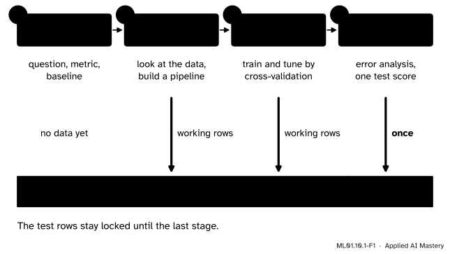
With the frame in place, a project runs through four stages. This module follows them, one lesson each.
ML01.10.1-F1
The four stages of a project and the rows each one may touch. The 89 test rows are opened once, in the last stage.
The bar keeps the project honest. A model must be judged on rows it has not seen (ML01.2), and even looking at the test rows while choosing spoils them (ML01.9.4). So they are set aside first.
Build it up
Step 1. Say who needs the prediction, and when. The clinic wants to plan the coming year at the first visit. So only what is known at that visit may be an input. The ten measurements qualify: age, sex, body mass index (BMI), average blood pressure and six blood serum measurements. Anything recorded later does not.
Step 2. Name the output and the kind of task. The output is the progression score one year on. It is a number, so this is regression (ML01.1.2).
Step 3. Choose the metric from the cost of an error. Say the model predicts 150 and the truth is 190. How bad is that, compared with being off by 20?
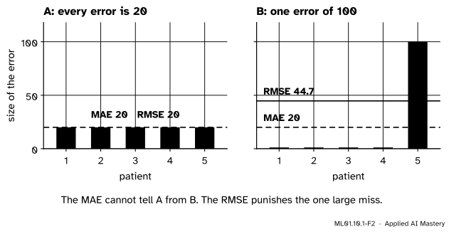
If an error twice as large is about twice as bad, the cost grows in step with the size of the error, and the metric that adds up sizes is the mean absolute error (MAE). If one large miss is far worse than several small ones, square the errors first: the root mean squared error (RMSE). ML01.7.4 defined both. Both are in points of the score.
ML01.10.1-F2
Two models with the same total error. The MAE scores them equally. The RMSE more than doubles for the model that put all its error on one patient.
This project assumes the clinic books follow-up visits in proportion to the predicted score (the study says nothing about costs), so an error of 40 points wastes or withholds about twice the care of an error of 20, in either direction. The cost is proportional, and this project’s metric is the MAE. The RMSE is reported beside it: a wide gap between the two signals a few very large errors.
Step 4. Set the baseline. The simplest prediction uses no input at all: one number for every patient. A model that cannot beat its score has learned nothing from the ten measurements. Which constant is best depends on the metric, as the next section shows.
Step 5. Fix the procedure before any result exists. The metric is chosen. Three more decisions are written down now, so that no result can bend them.
89 of the 442 patients are set aside as the test set, at random with a fixed seed.
Every candidate is scored by five-fold cross-validation (ML01.9.3) on the other 353.
The final model will be the simplest one whose score is within one standard error of the best.
The formal statement
NoteDefinition: prediction task
A prediction task is fixed by an input \(\vect{x}\) that is known when the prediction is made, an output \(y\) to be predicted, and a metric that scores predictions \(\hat{y}_i\) against targets \(y_i\). Its baseline is the best score of a constant prediction, \(\hat{y}_i = c\) for every \(i\).
Result 1 (from ML01.4.1): the best constant. Of all constant predictions, the mean of the targets has the lowest squared error, and so the lowest RMSE. A median has the lowest absolute error. So the baseline for the RMSE is the mean, and the baseline for the MAE is the median.
Result 2 (from ML01.7.4): the RMSE is never below the MAE. If \(V\) is the variance of the error sizes \(\abs{y_i - \hat{y}_i}\), then
\[
\text{RMSE}^2 = \text{MAE}^2 + V .
\]
The two are equal only when every error has the same size. The more uneven the errors, the wider the gap.
Result 3: unequal costs move the best constant. Suppose predicting too low costs \(u\) per point and predicting too high costs \(v\) per point. Let \(C(c)\) be the total cost of the constant \(c\), and slide \(c\) a small distance \(\delta\) to the right without crossing a target, as ML01.4.1 did for the median. Each of the \(\ell\) targets on the left of \(c\) was predicted too high, and is now too high by \(\delta\) more. Each of the \(r\) targets on the right was predicted too low, and is now too low by \(\delta\) less. So
Sliding right lowers the cost while \(v\,\ell < u\,r\) and raises it once \(v\,\ell > u\,r\). The cost is lowest where \(v\,\ell = u\,r\). Add \(u\,\ell\) to both sides to get \({(u + v)\,\ell} = {u\,(\ell + r)}\), that is
\[
\frac{\ell}{\ell + r} = \frac{u}{u + v} .
\]
The best constant has a fraction \({u/(u+v)}\) of the targets below it. Equal costs give one half, the median, and the total cost is then \(u\) times the total absolute error, a fixed multiple of the MAE. If predicting too low is three times as costly, the fraction is \(3/4\), the upper quartile. The cost of errors fixes the metric and the baseline together.
Result 4: skill is measured against the baseline. The share of the baseline’s error that a model removes is
\[
\text{skill} = 1 - \frac{\text{MAE of the model}}{\text{MAE of the baseline}} .
\]
It is \(0\) at the baseline and \(1\) for a perfect model. The \(R^2\) of ML01.7.4 is the same idea with squared errors and the mean as the baseline.
Go deeper: the models will be trained on squared error. Is that a mismatch?
A little. Linear regression and the lasso choose their weights to make the squared error small, which aims at the mean score of similar patients. The MAE rewards aiming at their median. Where scores are spread evenly about their centre, the two nearly coincide. And the comparison stays fair: every candidate, however it was trained, is scored by the MAE.
Worked example
The frame, written down.
Part
For the clinic
Input
Ten measurements from the first visit
Output
The progression score a year later
Metric
MAE, in points of the score
Baseline
The median of the training targets
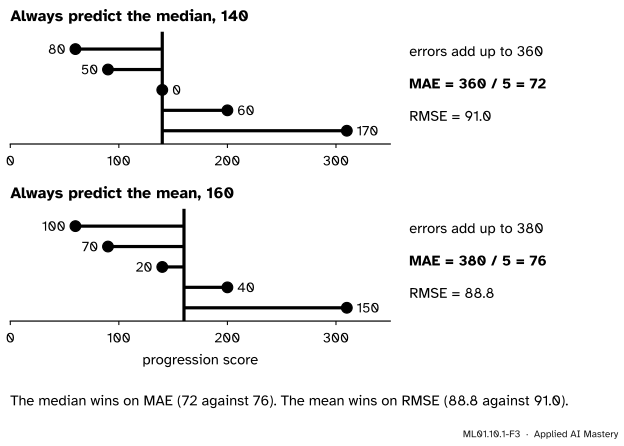
The baseline by hand. Take five of the working patients, chosen for their round scores: \(60, 90, 140, 200, 310\). Their median is the middle value, \(140\). Their mean is \(800 / 5 = 160\).
ML01.10.1-F3
The two constant guesses, scored on five patients. Each bar is one absolute error.
Guess the median, 140. The errors are \(80, 50, 0, 60, 170\). They add up to \(360\), so the MAE is \(360/5 = 72\). Their squares are \(6400, 2500, 0, 3600, 28900\), with mean \(41400/5 = 8280\), so the RMSE is \(\sqrt{8280} = 90.99\).
Guess the mean, 160. The errors are \(100, 70, 20, 40, 150\), total \(380\), so the MAE is \(76\). Their squares are \(10000, 4900, 400, 1600, 22500\), with mean \(39400/5 = 7880\), so the RMSE is \(\sqrt{7880} = 88.77\).
Each constant wins on its own metric, as Result 1 says. Result 2 holds too: for the median guess \(\text{MAE}^2 = 72^2 = 5184\), the variance of the sizes \(80, 50, 0, 60, 170\) is \(3096\), and their sum is \(8280 = \text{RMSE}^2\).
Unequal costs. Let too low cost \(3\) per point and too high cost \(1\). Result 3 asks for three quarters of the targets below \(c\). At \(c = 200\) three lie below and one above, and \({1 \times 3} = {3 \times 1}\). That guess is too high by \({140 + 110 + 60} = 310\) and too low by \(110\): cost \({310 + 3 \times 110} = 640\). The median, \(140\), is too high by \(130\) and too low by \(230\): cost \({130 + 690} = 820\).
Skill. A model with an MAE of \(54\) on these five patients would have skill \({1 - 54/72} = 0.25\): it removes a quarter of the baseline’s error.
Code
From scratch: the two metrics, the two constant guesses, and a search over every constant to check Results 1 and 3.
import numpy as npdef mae(y, y_hat):return np.mean(np.abs(y - y_hat))def rmse(y, y_hat):return np.sqrt(np.mean((y - y_hat) **2))five = np.array([60.0, 90.0, 140.0, 200.0, 310.0]) # five patients' progression scoresfor name, guess in [("median", np.median(five)), ("mean", five.mean())]:print(f"always predict the {name}, {guess:.0f}: MAE {mae(five, guess):.2f} RMSE {rmse(five, guess):.2f}")sizes = np.abs(five - np.median(five)) # 80, 50, 0, 60, 170print("MAE^2 + variance of the sizes:", sizes.mean() **2+ sizes.var(), " RMSE^2:", np.mean(sizes **2))grid = np.arange(0.0, 400.5, 0.5) # every constant from 0 to 400print("best constant for the MAE:", grid[np.argmin([mae(five, c) for c in grid])]," for the RMSE:", grid[np.argmin([rmse(five, c) for c in grid])])def cost(y, c, low=3.0, high=1.0): # low: the price of a point predicted too lowreturn np.sum(np.where(y > c, low * (y - c), high * (c - y)))print("costs 3 to 1, best constant:", grid[np.argmin([cost(five, c) for c in grid])]," cost there:", cost(five, 200.0), " at the median:", cost(five, 140.0))
always predict the median, 140:  MAE 72.00   RMSE 90.99
always predict the mean, 160:  MAE 76.00   RMSE 88.77
MAE^2 + variance of the sizes: 8280.0   RMSE^2: 8280.0
best constant for the MAE: 140.0   for the RMSE: 160.0
costs 3 to 1, best constant: 200.0   cost there: 640.0   at the median: 820.0
Now the real table, scikit-learn’s load_diabetes. The first line after loading sets the test rows aside. Nothing below it touches them.
from sklearn.datasets import load_diabetesfrom sklearn.model_selection import train_test_splitdata = load_diabetes(scaled=False) # the measurements in their own unitsX, y = data.data, data.targetX_work, X_test, y_work, y_test = train_test_split(X, y, test_size=89, random_state=10)print("table:", X.shape, " features:", ", ".join(data.feature_names))print("working rows:", len(y_work), " test rows, locked away:", len(y_test))print("the five patients, all working rows (143, 39, 374, 77 and 9 of the table):", y[[143, 39, 374, 77, 9]])print(f"working targets: {y_work.min():.0f} to {y_work.max():.0f}, median {np.median(y_work):.0f}, mean {y_work.mean():.1f}")
table: (442, 10)   features: age, sex, bmi, bp, s1, s2, s3, s4, s5, s6
working rows: 353   test rows, locked away: 89
the five patients, all working rows (143, 39, 374, 77 and 9 of the table): [ 60.  90. 140. 200. 310.]
working targets: 25 to 346, median 140, mean 152.9
The seed is 10, this module’s number. ML01.3.4 split the same table with seed 0 and looked at its test rows several times, so this project draws a fresh split and makes every choice without its test rows.
The baseline is scored the way every model will be, by five-fold cross-validation on the working rows: the constant is learned from four folds and scored on the fifth.
folds = np.array_split(np.arange(len(y_work)), 5) # five blocks of the shuffled working rowsdef cv_constant(pick, score=mae):"""Score 'always predict pick(training targets)' on each fold in turn.""" scores = []for held_out in folds: training = np.setdiff1d(np.arange(len(y_work)), held_out) guess = pick(y_work[training]) # learned without the held-out fold scores.append(score(y_work[held_out], guess))return np.array(scores)baseline = cv_constant(np.median)se = baseline.std(ddof=1) / np.sqrt(len(baseline))print("fold sizes:", [len(f) for f in folds])print("baseline MAE on each fold:", np.round(baseline, 2))print(f"baseline: {baseline.mean():.2f} +/- {se:.2f}")print(f"the mean as the guess: MAE {cv_constant(np.mean).mean():.2f}, RMSE {cv_constant(np.mean, rmse).mean():.2f}")print(f"the median as the guess: RMSE {cv_constant(np.median, rmse).mean():.2f}")
fold sizes: [71, 71, 71, 70, 70]
baseline MAE on each fold: [66.04 67.53 58.76 68.7  63.13]
baseline: 64.83 +/- 1.78
the mean as the guess: MAE 65.49, RMSE 76.51
the median as the guess: RMSE 77.55
The baseline is an MAE of \(64.83\), give or take a standard error of \(1.78\): the standard deviation of the five fold scores divided by \(\sqrt{5}\) (ML01.2.3). Result 1 holds on real data too. The median beats the mean on MAE, \(64.83\) against \(65.49\), and the mean beats the median on RMSE, \(76.51\) against \(77.55\).
The library version is DummyRegressor, a “model” that ignores its input. In scikit-learn a higher score is always better, so an error comes back negated.
from sklearn.dummy import DummyRegressorfrom sklearn.model_selection import KFold, cross_val_scorecv = KFold(n_splits=5) # the same five blocksscores =-cross_val_score(DummyRegressor(strategy="median"), X_work, y_work, cv=cv, scoring="neg_mean_absolute_error")r2 = cross_val_score(DummyRegressor(strategy="mean"), X_work, y_work, cv=cv, scoring="r2")print("scikit-learn, baseline MAE on each fold:", np.round(scores, 2))print(f"R squared of the mean baseline: {r2.mean():.3f}")for target in (45.0, 60.0):print(f"a model with MAE {target:.0f} would have skill {1- target / baseline.mean():.2f}")
scikit-learn, baseline MAE on each fold: [66.04 67.53 58.76 68.7  63.13]
R squared of the mean baseline: -0.007
a model with MAE 45 would have skill 0.31
a model with MAE 60 would have skill 0.07
The fold scores match. The \(R^2\) of the mean baseline is \(-0.007\), not \(0\), because the mean of four folds is not exactly the mean of the fifth. The bar is set: a model with an MAE of 45 would have a skill of \(0.31\).
Explore
This module’s interactive, the project board, is in lesson 3. It draws this lesson’s baseline as a dashed line and judges every pipeline you build against it.
Pitfalls
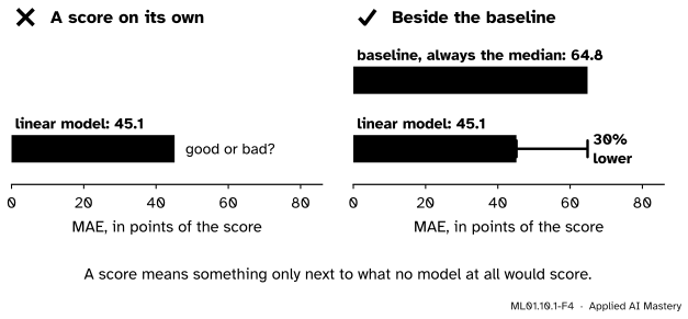
ML01.10.1-F4
Wrong beside right. The score \(45.1\) belongs to a model from lesson 3. Alone it says nothing. Beside the baseline it says: 30 percent of the error removed.
“An MAE of 45 sounds small, so the model is good.”
Small compared with what? On a target that hardly varied, the median alone might score \(10\). Compute the baseline first, with the same metric and the same rows.
“Use every column that helps the score.”
Only columns known at prediction time are inputs. A column filled in later, such as “treatment was intensified during the year”, would predict the score well and be useless at the first visit. No split can catch this kind of leak.
“The baseline for regression is the mean.”
For squared error, yes. For absolute error it is the median. Use the constant that is best for your metric, or the baseline is too weak and the model looks better than it is.
Check yourself
Recall
1. Which four things make up the frame of a prediction project?
Show answer
The input (what is known when predicting), the output (what is predicted), the metric (how an error is scored) and the baseline (the score of the best constant).
2. When is the MAE the right metric, and when the RMSE?
Show answer
The MAE when the cost of an error is proportional to its size. The RMSE when one large error is worse than several small ones of the same total.
3. Which constant prediction gives the lowest MAE, and which the lowest RMSE?
Show answer
The median of the targets gives the lowest MAE. The mean gives the lowest RMSE.
4. Predicting too low costs three times as much per point as predicting too high. Which constant is the best baseline?
Show answer
The one with a fraction \({3/(3+1)} = 3/4\) of the targets below it: the upper quartile.
5. What is this project’s baseline score, and how was it measured?
Show answer
An MAE of \(64.83\) with a standard error of \(1.78\): the median of the training targets, scored by five-fold cross-validation on the 353 working rows.
Exercises
1.★ Four houses sold for \(100\), \(120\), \(150\) and \(310\) thousand. Find the best constant prediction and its score (a) under MAE and (b) under RMSE.
Show solution
(a) Any constant between the two middle values, \(120\) and \(150\), is a median. Take \(135\): the errors are \(35, 15, 15, 175\), total \(240\), so the MAE is \(60\).
(b) The mean is \(680/4 = 170\). The errors are \(70, 50, 20, 140\), with squares \(4900, 2500, 400, 19600\) and mean \(27400/4 = 6850\). The RMSE is \(\sqrt{6850} = 82.8\).
2.★★ A model’s errors on six patients are \(10, -10, 10, -10, 10, -70\). A second model’s are \(20, -20, 20, -20, 20, -20\). Compute the MAE and the RMSE of each. Which model suits a clinic with proportional costs, and which a clinic for which one miss of 70 is a disaster?
Show solution
First model: the sizes are \(10, 10, 10, 10, 10, 70\), total \(120\), so the MAE is \(20\). The squares are \(100\) five times and \(4900\), total \(5400\), mean \(900\), so the RMSE is \(30\).
Second model: every size is \(20\), so the MAE is \(20\) and the RMSE is \(20\).
With proportional costs the two are equally good: the same MAE. If one large miss is a disaster, the RMSE is the guide and the second model wins, \(20\) against \(30\).
3.★★★ Predicting too low costs \(4\) per point and predicting too high costs \(1\). By Result 3, which constant should the baseline predict? Check on the targets \(10, 20, 30, 40, 50\) by computing the total cost at \(c = 30\), \(c = 40\) and \(c = 50\).
Show solution
With \(u = 4\) and \(v = 1\), a fraction \({u/(u+v)} = 4/5\) of the targets should lie below the constant. For five targets that is four: any \(c\) from \(40\) to \(50\).
At \(c = 30\): too high by \({20 + 10} = 30\) points, cost \(30\); too low by \({10 + 20} = 30\) points, cost \({4 \times 30} = 120\). Total \(150\).
At \(c = 40\): too high by \({30 + 20 + 10} = 60\), cost \(60\); too low by \(10\), cost \(40\). Total \(100\).
At \(c = 50\): too high by \({40 + 30 + 20 + 10} = 100\), cost \(100\); never too low. Total \(100\).
Both \(40\) and \(50\) cost \(100\), less than the median’s \(150\), as the rule predicts.
Summary card
Frame first: input, output, metric, baseline. Then lock the test rows away.
ML01.10.1-F1
Four stages; test rows opened once.
Metric. MAE if cost is proportional to the error; RMSE if large misses cost more.
Baseline. The best constant: the median for MAE, the mean for RMSE.
Unequal costs. The best constant has a fraction \({u/(u+v)}\) of the targets below it.
This project. 353 working rows, 89 test rows, baseline MAE \({64.83 \pm 1.78}\).
Sources and next steps
Sources. Each was opened and checked against this lesson on 12 November 2026.
Bradley Efron, Trevor Hastie, Iain Johnstone and Robert Tibshirani, Least Angle Regression, preprint of the 2004 paper in The Annals of Statistics. Section 1 and Table 1: ten baseline variables for \(n = 442\) diabetes patients, and a response that is “a quantitative measure of disease progression one year after baseline”.
scikit-learn 1.9 user guide. Section 9.1.2 lists the 442 instances and ten features. Section 3.4.6 defines the MAE and says that a constant model predicting the average gets an \(R^2\) of 0. Section 3.4.8 describes DummyRegressor and its median strategy.
Rob Hyndman and George Athanasopoulos, Forecasting: Principles and Practice, 3rd edition, Section 5.8: minimising the MAE leads to forecasts of the median, minimising the RMSE to forecasts of the mean.
Google, Introduction to Machine Learning Problem Framing, Framing an ML problem: the ideal outcome, the model’s output and success metrics.
Trevor Hastie, Robert Tibshirani and Jerome Friedman, The Elements of Statistical Learning, 2nd edition, Section 7.2, page 222: the test set should be kept in a “vault” and brought out only at the end of the analysis.