For two continuous variables the joint table becomes a surface with volume 1 beneath it, and the probability of a region is the volume above it: an integral inside an integral. Marginals, conditionals and independence carry over from the table, worked on a square and a triangle.
Describe a joint density as a surface with volume 1 beneath it, and the probability of a region as the volume above it.
Compute the probability of a region of the unit square as an integral inside an integral, slice by slice.
Find marginal and conditional densities by integrating out and dividing, in parallel with the joint table.
Test two continuous variables for independence by checking whether the density factorises everywhere.
Approximate a double integral with a Riemann sum on a grid, and compute it with scipy.integrate.dblquad.
In review. The maths and code on this page are checked by automated tests on every change, but an independent reader has not signed it off yet. Spot a mistake or a confusing step? Tell us.
The question
Pick a point at random in the unit square, every spot equally likely, and call its coordinates \(X\) and \(Y\). What is the chance that \({X + Y \leq 1}\)? No single point has any probability, so there is no table of cells to add up. Most features in machine learning are continuous like this: a height and a weight, two pixel intensities, two coordinates of an embedding. How do we describe two of them together?
From the last lesson
1. How do you get \({p(y \mid x)}\) from a joint table, and what are the conditional means on the course’s table?
Show answer
Divide row \(x\) by its total \({p_X(x)}\). The means are \(1/2\), \(1\) and \(3/2\) for \({x = 0, 1, 2}\).
2. When are two discrete variables independent, in terms of rows?
Show answer
When every row with positive total rescales to the same PMF, which is then \(p_Y\).
Intuition
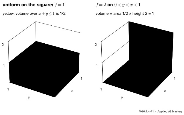
For one continuous variable, a density was a curve and probability was the area under it (M06.6.1). For two, the density is a surface over the plane: a height \({f(x, y)}\) above each point. Probability is the volume under the surface, and the whole volume is 1.
M06.9.4-F1
Two joint densities. Left: height 1 over the whole square, with the region \({x + y \leq 1}\) in yellow. Right: height 2 over a triangle. Each has volume 1 under it.
On the left, the yellow block sits on half the square at height 1, so its volume is \(1/2\). That is \({\Prob(X + Y \leq 1)}\), the answer to the question. The right-hand density is twice as tall on half the area, which keeps the total volume at 1.
Build it up
Step 1. The height is a density, not a probability. As in one dimension, a single point has probability 0. A tiny square of sides \(\Delta x\) and \(\Delta y\) near \({(x, y)}\) has probability close to \({f(x, y)\,\Delta x\,\Delta y}\): height times base area. That is why \(f\) can be 2 without anything going wrong.
Step 2. A region’s probability is the volume above it. Cover the region with tiny squares, add their volumes, and let the squares shrink. The limit is the volume under the surface and above the region.
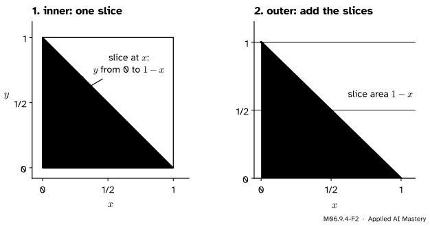
Step 3. Find the volume one slice at a time. Fix \(x\) and cut the solid along the line at that \(x\). The cut is a flat slice; its area is an ordinary integral in \(y\). Then add the slice areas across \(x\) with a second ordinary integral. One integral sits inside the other.
M06.9.4-F2
The inner integral gives the area of the slice at \(x\); the outer integral adds the slice areas. For the uniform density each slice has area \({1 - x}\), and the area under that line is \(1/2\).
Step 4. Do it for the square. With \({f = 1}\), the slice at \(x\) runs from \({y = 0}\) to \({y = 1 - x}\), so its area is
\[
\int_0^{1-x} 1\, dy = 1 - x.
\]
Adding the slices from \({x = 0}\) to 1 (with the antiderivative from M04.6):
Taking \(R\) to be the whole plane gives \({\iint f = 1}\): the volume under the surface is 1.
For a region whose slices are intervals, \({a \leq x \leq b}\) and \({g(x) \leq y \leq h(x)}\), the double integral is an iterated integral, one inside the other:
\[
\iint_R f \;=\; \int_a^b \bigg( \int_{g(x)}^{h(x)} f(x, y)\, dy \bigg) dx .
\]
Inside, \(x\) is held fixed and \(y\) runs along the slice; the result is a function of \(x\), which the outside integral adds up. The limits of the inside integral follow the edge of the region, so they may depend on \(x\). Module M05.6 treats double integrals in full, over regions of any shape.
Marginal densities. For an interval of \(x\) values,
\[
\begin{aligned}
&\Prob(a \leq X \leq b) \\
&= \int_a^b \bigg( \int f(x, y)\, dy \bigg) dx,
\end{aligned}
\]
taking every \(y\). So the inner integral does for \(X\) exactly what a density does: integrated over an interval, it gives the probability. It is the marginal density:
Conditional densities. Where \({f_X(x) > 0}\), the conditional density of \(Y\) given \({X = x}\) is the slice rescaled to area 1:
\[
f(y \mid x) = \frac{f(x, y)}{f_X(x)}.
\]
Independence.\(X\) and \(Y\) are independent when \({f(x, y) = f_X(x)\, f_Y(y)}\) for every \(x\) and \(y\): the density factorises. As with tables, this holds exactly when every slice rescales to the same density.
Every idea of the module carries over, with sums turned into integrals:
Table
Density
Total
\({\sum\sum p = 1}\)
\({\iint f = 1}\)
\(p_X\), \(f_X\)
\({\sum_y p}\)
\({\int f\, dy}\)
Given \(x\)
\({p / p_X}\)
\({f / f_X}\)
Independent
\({p = p_X\, p_Y}\)
\({f = f_X\, f_Y}\)
Go deeper: why the conditional density is a slice rescaled
In the table, conditioning on \({X = x}\) kept a row and divided by its total. Here the event \({X = x}\) has probability 0, so the definition of M06.3.1 cannot be used directly. Condition instead on the thin strip \({x \leq X \leq x + \Delta x}\), which has probability close to \({f_X(x)\,\Delta x}\). The part of the strip with \({c \leq Y \leq d}\) has probability close to \({\Delta x \int_c^d f(x, y)\, dy}\). Dividing, \(\Delta x\) cancels and leaves \({\int_c^d f(x, y)/f_X(x)\, dy}\). As the strip narrows, this is the integral of \({f(y \mid x)}\) over \({[c, d]}\). Making this limit rigorous is left to later courses.
Worked example
The density 2 on the triangle \({0 < y < x < 1}\). Check that it is a density, then find its marginals, its conditionals and whether \(X\) and \(Y\) are independent.
Total volume. For each \(x\) the slice runs from \({y = 0}\) up to the diagonal \({y = x}\):
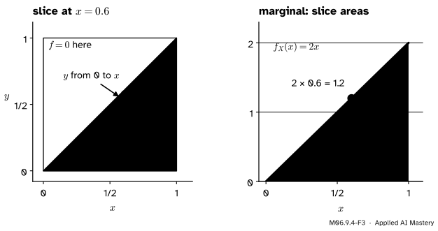
Marginal of \(X\). The inner integral is already it: \({f_X(x) = \int_0^x 2\, dy = 2x}\) on \({[0, 1]}\). That is the course’s hand density, with mean \(2/3\) (M06.7.1).
M06.9.4-F3
The slice at \({x = 0.6}\) is 0.6 long and 2 high, so its area is 1.2. Slice areas across \(x\) trace out the marginal \({f_X(x) = 2x}\).
Marginal of \(Y\). Now fix \(y\): the slice runs across from \({x = y}\) to \({x = 1}\), so \({f_Y(y) = \int_y^1 2\, dx = 2(1 - y)}\) on \({[0, 1]}\). It leans the other way: \(Y\) is usually small.
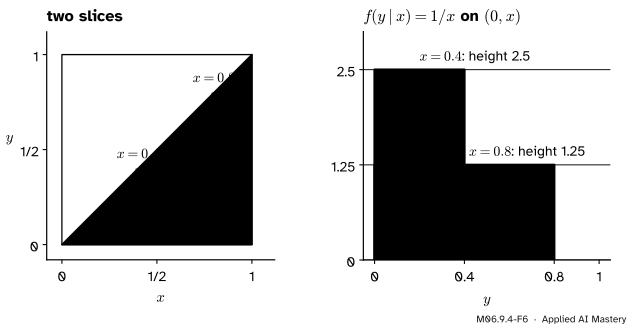
Conditional of \(Y\) given \({X = x}\). For \({0 < x \leq 1}\),
and 0 elsewhere. That is \({\mathrm{Unif}(0, x)}\): given \(X\), \(Y\) is equally likely to be anywhere below it, and \({\E[Y \mid X = x] = x/2}\).
M06.9.4-F6
Each slice, rescaled to area 1, is a uniform density on \({(0, x)}\). Short slices become tall rectangles. The shape changes with \(x\), so \(X\) and \(Y\) are not independent.
Independence. The slices change with \(x\), so the variables are dependent. A single point shows it: \({f(0.25, 0.5) = 0}\), because that point lies above the diagonal, but \({f_X(0.25)\,f_Y(0.5)} = {0.5 \times 1} = {0.5}\). For the uniform square, by contrast, \({f_X(x) = \int_0^1 1\, dy = 1}\) and likewise \({f_Y(y) = 1}\), so \({f = 1 = f_X\, f_Y}\) everywhere: independent.
Code
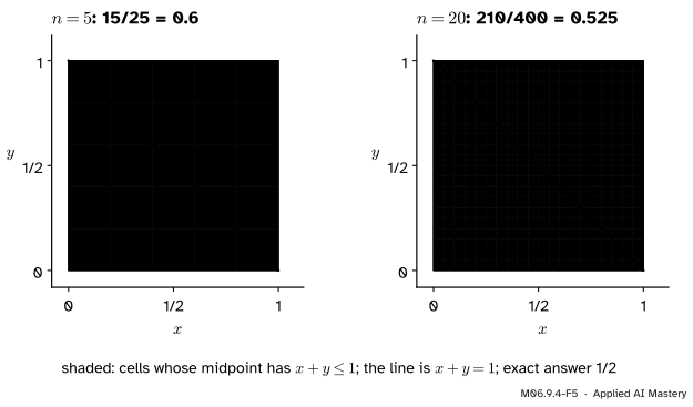
From scratch, a midpoint Riemann sum on an \(n\) by \(n\) grid: each small square contributes its height at the midpoint times its area \({1/n^2}\).
import numpy as npdef riemann_2d(f, region, n):"""Midpoint sum of f over the part of the unit square where region(x, y) is True.""" mid = (np.arange(n) +0.5) / n x, y = np.meshgrid(mid, mid, indexing="ij") # x along axis 0, y along axis 1returnfloat(np.sum(f(x, y) * region(x, y)) / n **2)uniform =lambda x, y: np.ones_like(x)triangle =lambda x, y: np.where(y < x, 2.0, 0.0)below_line =lambda x, y: x + y <=1everywhere =lambda x, y: np.ones_like(x, dtype=bool)for n in (5, 20, 1000):print(n, "P(X + Y <= 1) ~", riemann_2d(uniform, below_line, n))print("triangle volume ~", riemann_2d(triangle, everywhere, 1000))
5 P(X + Y <= 1) ~ 0.6
20 P(X + Y <= 1) ~ 0.525
1000 P(X + Y <= 1) ~ 0.5005
triangle volume ~ 0.999
M06.9.4-F5
The grid’s staircase overshoots the triangle a little; the overshoot shrinks as the grid gets finer. With \(n\) cells a side the sum is \({(n + 1)/(2n)}\): 0.6, 0.525, then 0.5005.
The sums approach \(1/2\) from above. The line cuts \(n\) cells in half, and their midpoints lie exactly on it, so each counts in full: an overshoot of \({n \times \tfrac12 \times \tfrac{1}{n^2}} = {\tfrac{1}{2n}}\).
scipy.integrate.dblquad does the iterated integral directly. Its function takes \(y\)first, and the inner limits are functions of \(x\).
\({\Prob(X \leq 1/2)} = {1/4}\) agrees with the hand density’s CDF \(x^2\) at \(1/2\). Last, a simulation. The larger and the smaller of two independent \({\mathrm{Unif}(0, 1)}\) numbers have exactly the triangle density (exercise 3 asks why), so they give samples to check the conditional mean \({x/2}\) against.
rng = np.random.default_rng(4)u = rng.random((200_000, 2))X, Y = u.max(axis=1), u.min(axis=1) # a point of the triangle densitynear = np.abs(X -0.6) <0.01# a thin strip around x = 0.6print("P(X + Y <= 1) ~", round(float(np.mean(X + Y <=1)), 3))print("mean of Y in the strip ~", round(float(Y[near].mean()), 3), " (x/2 = 0.3)")
P(X + Y <= 1) ~ 0.5
mean of Y in the strip ~ 0.303  (x/2 = 0.3)
Explore
The joint table explorer is in lesson M06.9.3. Each row it rescales is the discrete version of a slice here: keep the slice, divide by its total.
Pitfalls
M06.9.4-F4
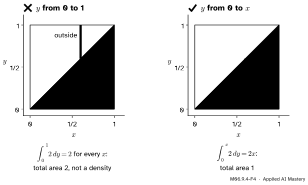
Wrong beside right. The inner limits must stop where the density stops. Running \(y\) up to 1 pretends the density is 2 where it is 0.
“The inner integral always runs over the whole range of \(y\).”
Only when the region is a rectangle. Over the triangle, \({\int_0^1 2\, dy = 2}\) for every \(x\) gives a “marginal” with area 2. The formula \({f = 2}\) holds only below the diagonal; above it \(f\) is 0. The inner limits follow the region: \({y}\) from 0 to \(x\).
“A joint density of 2 means a probability of 2.”
The height is probability per unit area. \({f = 2}\) on the triangle means a small square of area \({0.01}\) near a point of the triangle has probability about \(0.02\). Only volumes are probabilities.
“\({f(x, y) = 2}\) is a constant, so it factorises and \(X\) and \(Y\) are independent.”
The density must factorise everywhere, including where it is 0. The triangle density is 2 on the triangle and 0 off it, and that edge \({y < x}\) ties the two variables together. If \({f = f_X\, f_Y}\), then \(f\) is positive exactly where \({f_X(x)}\) and \({f_Y(y)}\) are both positive; when each marginal is positive on an interval, that region is a rectangle. A triangle is not one.
Check yourself
Recall
1. In the picture of a joint density, what is the probability of a region?
Show answer
The volume under the surface \({z = f(x, y)}\) and above the region.
2. What does the inner integral of \({\int_a^b \big( \int_{g(x)}^{h(x)} f\, dy \big) dx}\) compute?
Show answer
The area of the slice of the solid at a fixed \(x\), with \(y\) running across the region from \({g(x)}\) to \({h(x)}\).
3. How do you get \({f_X}\) from a joint density?
Show answer
Integrate out \(y\): \({f_X(x) = \int f(x, y)\, dy}\), the area of the slice at \(x\).
4. For the density 2 on \({0 < y < x < 1}\), what is the conditional density of \(Y\) given \({X = x}\)?
Show answer
\({1/x}\) on \({0 < y < x}\): the uniform density on \({(0, x)}\).
5. In scipy.integrate.dblquad(func, a, b, gfun, hfun), which argument does func take first, and what are gfun and hfun?
Show answer
func(y, x) takes \(y\) first. gfun and hfun give the lower and upper limits of \(y\) as functions of \(x\) (or constants); \(x\) runs from a to b.
Exercises
1.★\(X\) and \(Y\) are uniform on the unit square. Find \({\Prob(Y \leq X^2)}\).
Show solution
The slice at \(x\) runs from \({y = 0}\) to \({y = x^2}\), so its area is \({\int_0^{x^2} 1\, dy = x^2}\). Adding the slices: \({\int_0^1 x^2\, dx} = {\big[x^3/3\big]_0^1} = {1/3}\).
2.★★ For the density 2 on \({0 < y < x < 1}\), find \({\Prob(X + Y \leq 1)}\).
Show solution
The slice at \(x\) runs from \({y = 0}\) to whichever comes first, the diagonal \({y = x}\) or the line \({y = 1 - x}\). For \({x \leq 1/2}\) that is \(x\); for \({x \geq 1/2}\) it is \({1 - x}\). So
Each piece is the area of a triangle with base \(1/2\) and height 1.
3.★★★ Let \(U\) and \(V\) be independent \({\mathrm{Unif}(0, 1)}\) numbers, and let \({X = \max(U, V)}\) and \({Y = \min(U, V)}\). Show that for any region \(R\) inside the triangle \({0 < y < x < 1}\), \({\Prob((X, Y) \in R)}\) is twice the area of \(R\), so \({(X, Y)}\) has the density 2 on the triangle.
Show solution
\({(U, V)}\) is uniform on the square, with density \({1 \times 1 = 1}\) because the two are independent. \({(X, Y)}\) lands in \(R\) when either \({(U, V)}\) lands in \(R\) (the case \({U > V}\)) or \({(V, U)}\) lands in \(R\) (the case \({V > U}\)); ties have probability 0. The second case is \({(U, V)}\) landing in \(R'\), the mirror image of \(R\) in the diagonal. \(R\) and \(R'\) lie on opposite sides of the diagonal, so they do not overlap, and both have the same area as \(R\). With density 1 on the square, \({\Prob((X, Y) \in R)} = {\text{area}(R) + \text{area}(R')} = {2\,\text{area}(R)}\), which is the integral of 2 over \(R\).
Summary card
Probability is volume under the density surface.
M06.9.4-F1
Volume 1 under each surface.
Joint density.\({f \geq 0}\), \({\iint f = 1}\), and \({\Prob((X, Y) \in R) = \iint_R f}\).
Iterated integral. Inner over the slice at \(x\), outer over \(x\).
Independent exactly when \({f = f_X\, f_Y}\) everywhere.
Examples. Uniform square: \({\Prob(X + Y \leq 1) = 1/2}\). Density 2 on the triangle: \({f_X(x) = 2x}\) and \({Y \mid X = x}\) is \({\mathrm{Unif}(0, x)}\).
Sources and next steps
Sources. Each was opened and checked against this lesson on 12 November 2026.
Hossein Pishro-Nik, Introduction to Probability, Statistics, and Random Processes, Section 5.2.1: the joint PDF as a non-negative function with \({P((X, Y) \in A) = \iint_A f_{XY}\, dx\, dy}\) (equation 5.15), total integral 1, and the marginals \({f_X(x) = \int f_{XY}(x, y)\, dy}\); its third example is a density on the triangle \({0 \leq y \leq x \leq 1}\). Section 5.2.3 gives the conditional PDF \({f_{X|Y}(x \mid y) = f_{XY}(x, y)/f_Y(y)}\) and independence as \({f_{XY}(x, y) = f_X(x)f_Y(y)}\) for all \(x\), \(y\).
MIT OpenCourseWare 18.05, Reading 7a, Joint Distributions, Independence, Spring 2022. Section 3.2: a small rectangle near \({(x, y)}\) has probability \({f(x, y)\,dx\,dy}\), and a joint pdf can be greater than 1. Section 3.3, Example 4: for the uniform density on the unit square the event \({X > Y}\) has probability \(0.5\). Section 3.8 gives marginal pdfs by integrating out, and Section 3.10 pictures probability as the volume under the surface.
SciPy reference, scipy.integrate.dblquad: dblquad(func, a, b, gfun, hfun) integrates func(y, x), with \(y\) the first argument, for \(x\) from a to b and \(y\) from gfun(x) to hfun(x), and returns the value with an error estimate.
Next. M06.10.1 multiplies by \({x\,y}\) under the joint table to measure how two variables move together. Module M05.6 treats double integrals in full, and M07.3 meets the most important joint density of all, the bivariate normal.