Bernoulli, binomial, geometric, Poisson, uniform, exponential, normal and categorical on one map, with arrows for how one becomes another. Choose a family for data by its story, see what goes wrong when the story does not fit, and meet the categorical distribution behind a softmax.
Give the story, parameters, mean and variance of each family of the course.
Explain each arrow of the map: adding Bernoullis, the binomial-to-Poisson and geometric-to-exponential limits, the normal for many trials, and the inverse CDF.
Choose a family for a variable from its story, and recognise when the story does not fit.
Describe the categorical distribution, draw from it, and connect it to the softmax output of a classifier.
Build each family in scipy.stats with the right parameters.
In review. The maths and code on this page are checked by automated tests on every change, but an independent reader has not signed it off yet. Spot a mistake or a confusing step? Tell us.
The question
A data set has five columns: correct answers out of 50 on a quiz, support tickets in each hour, minutes between tickets, a sensor’s measurement error, and the class a network gives an image. Which distribution should model each one? The answer comes from how each number is made, its story, and not from the shape of a histogram.
From the last lesson
1. Which binomials does \({\mathrm{Pois}(\lambda)}\) approximate?
Show answer
\({\mathrm{Bin}(n, p)}\) with \(n\) large, \(p\) small and \({np = \lambda}\).
2. What are the mean and variance of \({\mathrm{Pois}(\lambda)}\)?
Show answer
Both are \(\lambda\).
Intuition
The families of this course are not a list to memorise. They are a few stories, and the stories are joined: one family turns into another when you add copies, shrink a step or pass a number through a function.
M06.8.4-F1
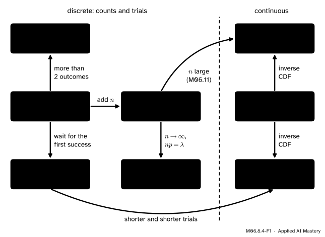
The map of the families. Each box is a story; each arrow is a way one story becomes another.
At the centre is the Bernoulli trial, one yes or no. Add \(n\) of them and you get a binomial. Wait for the first yes and you get a geometric. Give the trial more than two outcomes and you get a categorical. The other arrows are limits, and one is a recipe.
Build it up
Step 1. Add Bernoullis: binomial. A sum of \(n\) independent \({\mathrm{Bern}(p)}\) indicators is \({\mathrm{Bin}(n, p)}\) (M06.8.1).
Step 2. Many unlikely trials: Poisson.\({\mathrm{Bin}(n, \lambda/n) \to \mathrm{Pois}(\lambda)}\) as \({n \to \infty}\) (M06.8.3).
Step 3. Shorter and shorter trials: exponential. A geometric wait in slots of length \({1/n}\), each with chance \({\lambda/n}\), tends to \({\mathrm{Exp}(\lambda)}\) (M06.8.2).
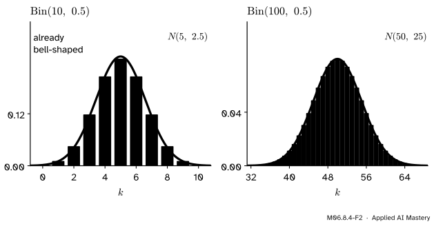
Step 4. Many trials: the normal. Keep \(p\) fixed and let \(n\) grow. The binomial bars take on the bell shape of the normal density with the same mean \({np}\) and variance \({np(1 - p)}\).
M06.8.4-F2
Binomial bars with the normal curve of the same mean and variance in vermillion. Already at \({n = 10}\) the fit is close; at \({n = 100}\) the curve runs through the tops of the bars.
This is the central limit theorem at work, shown here and stated in M06.11: a sum of many small independent pieces is close to normal, whatever the pieces are.
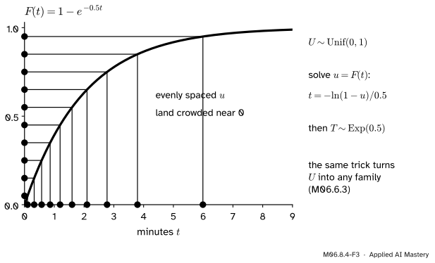
Step 5. A uniform number through the inverse CDF: anything. M06.6.3 showed that if \({U \sim \mathrm{Unif}(0, 1)}\) and \(F\) is a CDF, then \({F^{-1}(U)}\) has CDF \(F\). For the exponential, solve \({u = 1 - e^{-\lambda t}}\) for \(t\):
\[
t = F^{-1}(u) = -\frac{\ln(1 - u)}{\lambda} .
\]
Check it directly. For \({t \ge 0}\), since \({\ln}\) is increasing,
The inverse CDF as a machine. Evenly spaced uniform numbers, read across to the CDF and down, crowd where the density is high: the waiting times come out exponential.
This is how computers sample every family: start from uniform numbers and transform them.
The formal statement
NoteThe families of the course, with their stories
Bernoulli\({\mathrm{Bern}(p)}\): one trial; 1 for success, 0 for failure.
Geometric\({\mathrm{Geom}(p)}\): trials up to and including the first success; values \({1, 2, \ldots}\).
Poisson\({\mathrm{Pois}(\lambda)}\): events in a window, from many unlikely chances; values \({0, 1, 2, \ldots}\).
Uniform\({\mathrm{Unif}(a, b)}\): a point with no preference anywhere in \({[a, b]}\).
Exponential\({\mathrm{Exp}(\lambda)}\): the wait for the next event at rate \(\lambda\); values \({t \ge 0}\).
Normal\({N(\mu, \sigma^2)}\): a sum of many small independent effects; any real value.
Categorical\({\mathrm{Cat}(p_1, \ldots, p_K)}\): one label out of \(K\), label \(k\) with chance \(p_k\).
The means and variances of the discrete families:
Family
Mean
Variance
\({\mathrm{Bern}(p)}\)
\(p\)
\({p(1-p)}\)
\({\mathrm{Bin}(n, p)}\)
\({np}\)
\({np(1-p)}\)
\({\mathrm{Geom}(p)}\)
\({1/p}\)
\({(1-p)/p^2}\)
\({\mathrm{Pois}(\lambda)}\)
\(\lambda\)
\(\lambda\)
And of the continuous ones:
Family
Mean
Variance
\({\mathrm{Unif}(a, b)}\)
\({(a+b)/2}\)
\({(b-a)^2/12}\)
\({\mathrm{Exp}(\lambda)}\)
\({1/\lambda}\)
\({1/\lambda^2}\)
\({N(\mu, \sigma^2)}\)
\(\mu\)
\({\sigma^2}\)
The categorical distribution. A categorical variable takes one of \(K\) labels, with chances \({p_1, \ldots, p_K}\) that are never negative and add to 1. With \({K = 2}\) it is a Bernoulli, with the labels written 1 and 0. Its labels need not be numbers, so it has no mean of its own. Write it instead as a one-hot vector\(\vect{y}\), with a 1 in the place of the label drawn and 0 elsewhere. Each entry \(y_k\) is the indicator of label \(k\), so \({\E[y_k] = p_k}\), and the mean of the one-hot vector is the probability vector \({(p_1, \ldots, p_K)}\).
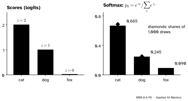
A classifier with \(K\) classes outputs exactly this. Its last layer gives scores \({z_1, \ldots, z_K}\) (logits), and the softmax turns them into a categorical distribution:
Every \(p_k\) is positive and they add to 1, whatever the scores (ML01.6.4).
M06.8.4-F6
The softmax turns the scores \({(2, 1, 0)}\) into the categorical distribution \({(0.665, 0.245, 0.090)}\). The blue diamonds are the shares of each class in 1,000 draws from it.
The families in SciPy. Each is an object in scipy.stats, and the parameter names differ from the textbook ones in four places (Poisson, uniform, exponential and normal):
Family
SciPy name
Parameters
\({\mathrm{Bern}(p)}\)
bernoulli
p
\({\mathrm{Bin}(n, p)}\)
binom
n, p
\({\mathrm{Geom}(p)}\)
geom
p
\({\mathrm{Pois}(\lambda)}\)
poisson
mu\({= \lambda}\)
\({\mathrm{Unif}(a, b)}\)
uniform
loc\({= a}\), scale\({= b - a}\)
\({\mathrm{Exp}(\lambda)}\)
expon
scale\({= 1/\lambda}\)
\({N(\mu, \sigma^2)}\)
norm
loc\({= \mu}\), scale\({= \sigma}\)
SciPy has no separate categorical object: draw one with rng.choice(K, p=probs) in NumPy, or use scipy.stats.multinomial(1, probs), which gives the one-hot vector.
Worked example
Choose a family for each column of the opening data set, and compute one number for each.
M06.8.4-F4
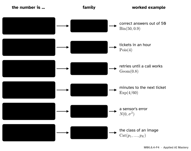
Choosing by the story. Ask how the number is made, follow the row to the family, then fill in the parameters from what you know.
Correct answers out of 50. A fixed number of questions, each right with about the same chance, say 0.9: \({\mathrm{Bin}(50, 0.9)}\). Mean \({50 \times 0.9 = 45}\), standard deviation \({\sqrt{50 \times 0.9 \times 0.1} = \sqrt{4.5} = 2.12}\).
Tickets in an hour, 4 on average. Many customers, each unlikely to write in a given hour: \({\mathrm{Pois}(4)}\). An hour with no ticket has chance \({e^{-4} = 0.0183}\).
Minutes to the next ticket. The same stream seen as a wait, at rate \({4/60 = 1/15}\) per minute: \({\mathrm{Exp}(1/15)}\), mean 15 minutes, and a gap of more than half an hour has chance \({e^{-30/15} = e^{-2} = 0.1353}\).
Retries until a call to a flaky service works, each call working with chance 0.8: \({\mathrm{Geom}(0.8)}\), mean \({1/0.8 = 1.25}\) calls, and needing more than 2 calls has chance \({0.2^2 = 0.04}\).
A sensor’s error, the sum of many small disturbances: \({N(0, \sigma^2)}\), with \(\sigma\) found by calibration. The class of an image: categorical, with the probabilities from a softmax.
Code
From scratch: an inverse-CDF sampler for the exponential, and a check of the mean and variance of every family in the tables by simulation.
Last, the SciPy objects with the parameters of the third table, each asked for its mean and variance:
from scipy import statsfamilies = {"bernoulli": stats.bernoulli(0.3), "binom": stats.binom(50, 0.9), "geom": stats.geom(0.8),"poisson": stats.poisson(mu=4), "uniform": stats.uniform(loc=2, scale=5-2),"expon": stats.expon(scale=15), "norm": stats.norm(loc=1, scale=2),}for name, dist in families.items():print(f"{name:9} mean {dist.mean():7.4f} variance {dist.var():8.4f}")print(stats.multinomial(1, p).rvs(random_state=0))
bernoulli mean  0.3000  variance   0.2100
binom     mean 45.0000  variance   4.5000
geom      mean  1.2500  variance   0.3125
poisson   mean  4.0000  variance   4.0000
uniform   mean  3.5000  variance   0.7500
expon     mean 15.0000  variance 225.0000
norm      mean  1.0000  variance   4.0000
[[1 0 0]]
The last line prints one draw from multinomial(1, p): a one-hot vector with a single 1.
Explore
M06.8-X1
Distribution map
Choose a family to see its PMF or density, with sliders for its parameters and the mean and one standard deviation either side marked in orange. Then choose an arrow and step \(n\) up: watch a binomial with \({np}\) fixed settle onto a Poisson, a geometric staircase onto an exponential, or binomial bars onto a normal curve.
Pitfalls
M06.8.4-F5
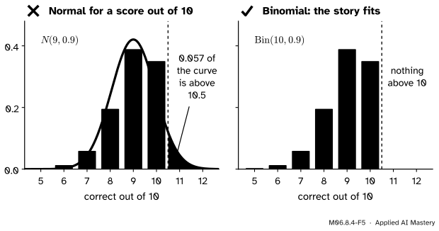
Wrong beside right. A normal curve with the right mean and variance still puts 5.7% of its probability on scores above 10.5, which cannot happen. The binomial story fits the score exactly.
“The histogram looks like a bell, so the data are normal.”
A score out of 10 can look bell-shaped, but it is a whole number between 0 and 10, and a normal model puts probability above 10, below 0 and between the whole numbers. Choose the family by the story of the number; use the normal as an approximation, knowing where it fails.
“Waits and counts are interchangeable.”
The minutes between tickets and the tickets per hour come from the same stream, but they are different numbers with different families: an exponential wait and a Poisson count. Mixing them up gives answers in the wrong units, such as a mean of 4 minutes where 15 was right.
“A softmax output is \(K\) separate yes or no probabilities.”
A categorical distribution picks exactly one label, so its probabilities add to 1: raising one lowers the others. When an image may hold a cat and a dog at once, the task needs \(K\) separate Bernoulli variables, one sigmoid per label, whose chances need not add to 1.
Check yourself
Recall
1. Which arrow turns a geometric into an exponential?
Show answer
Shorter and shorter trials: slots of length \({1/n}\) with chance \({\lambda/n}\) each, as \({n \to \infty}\).
2. Give the mean and variance of \({\mathrm{Unif}(a, b)}\) and of \({\mathrm{Exp}(\lambda)}\).
Show answer
\({(a + b)/2}\) and \({(b - a)^2/12}\); \({1/\lambda}\) and \({1/\lambda^2}\).
3. How do you turn \({U \sim \mathrm{Unif}(0, 1)}\) into an \({\mathrm{Exp}(\lambda)}\) wait?
Show answer
\({T = -\ln(1 - U)/\lambda}\), the inverse of the CDF \({1 - e^{-\lambda t}}\).
4. What is the categorical distribution, and where does it appear in machine learning?
Show answer
One label out of \(K\), label \(k\) with chance \(p_k\); the softmax output of a \(K\)-class classifier is a categorical distribution.
5. How do you build \({N(\mu, \sigma^2)}\) and \({\mathrm{Unif}(a, b)}\) in scipy.stats?
Show answer
norm(loc=mu, scale=sigma), with the standard deviation as scale; uniform(loc=a, scale=b - a).
Exercises
1.★ Show that \({\mathrm{Var}(U) = 1/12}\) for \({U \sim \mathrm{Unif}(0, 1)}\), and deduce the variance of \({\mathrm{Unif}(a, b)}\).
Show solution
\({\E[U] = \int_0^1 u\,du = \tfrac12}\) and \({\E[U^2] = \int_0^1 u^2\,du = \tfrac13}\), so \({\mathrm{Var}(U) = \tfrac13 - \tfrac14 = \tfrac{1}{12}}\). The variable \({X = a + (b - a)U}\) is \({\mathrm{Unif}(a, b)}\), and \({\mathrm{Var}(cU + a) = c^2\,\mathrm{Var}(U)}\) (M06.7.3), so \({\mathrm{Var}(X) = (b - a)^2/12}\).
2.★★ Emails reach an inbox at 0.2 per minute. Name the family and parameter of (a) the number of emails in an hour, (b) the minutes until the next email, (c) the number of sixes in 30 rolls of a die. Give each mean.
Show solution
(a) A count in a window: \({\mathrm{Pois}(0.2 \times 60) = \mathrm{Pois}(12)}\), mean 12.
(b) A wait in continuous time: \({\mathrm{Exp}(0.2)}\), mean \({1/0.2 = 5}\) minutes, which SciPy writes expon(scale=5).
(c) Successes in a fixed number of trials: \({\mathrm{Bin}(30, 1/6)}\), mean 5.
3.★★★ Two servers receive requests independently, the first after a wait \({S \sim \mathrm{Exp}(a)}\) and the second after \({T \sim \mathrm{Exp}(b)}\). Show that the wait until the first of them receives one, \({\min(S, T)}\), is \({\mathrm{Exp}(a + b)}\).
Show solution
The minimum is above \(t\) exactly when both waits are above \(t\). By independence,
which is the tail of \({\mathrm{Exp}(a + b)}\). Rates add: two streams at 0.5 per minute each give a first request after 1 minute on average.
Summary card
Choose a family by its story; the arrows say how the stories are joined.
M06.8.4-F1
Eight families, one map.
Count out of \(n\): binomial. Count in a window: Poisson.
Wait in trials: geometric. Wait in time: exponential.
Sum of many small effects: normal. One label of \(K\): categorical.
Any family from a uniform number through the inverse CDF.
Sources and next steps
Sources. Each was opened and checked against this lesson on 12 November 2026.
Hossein Pishro-Nik, Introduction to Probability, Statistics, and Random Processes, Section 3.1.5 (the Bernoulli, geometric, binomial and Poisson distributions, the binomial as a sum of Bernoullis and the Poisson as a limit of binomials) and Section 4.2.2 (the exponential as a limit of geometric waits).
SciPy developers, Statistical functions (scipy.stats) (SciPy 1.18 reference), which lists bernoulli, binom, geom and poisson among the discrete distributions, uniform, expon and norm among the continuous ones, and multinomial among the multivariate ones; norm takes the mean as loc and the standard deviation as scale, and uniform is the uniform distribution on \({[\text{loc}, \text{loc} + \text{scale}]}\).
NumPy developers, Generator.choice (NumPy 2.5 reference), whose p gives the probabilities associated with each entry.
Next. M06.9 puts two random variables on one table and asks how they move together; M06.11 states the arrow to the normal, the central limit theorem, and shows it at work; and ML01.6.4 uses the categorical distribution for classifiers with more than two classes.