The variance is the expected squared distance from the mean and the standard deviation is its square root, in the units of X. Derive the shortcut E[X²] − (E[X])², how shifts, stretches and independent sums change the spread, and why the spread of a sum grows like √n.
Define the variance as the expected squared distance from the mean, and the standard deviation as its square root in the units of X.
Derive the shortcut Var(X) = E[X²] − (E[X])² and use it for a die, a Bernoulli variable, the sum of two dice and the density 2x.
Derive Var(aX + b) = a²Var(X), and Var(X + Y) = Var(X) + Var(Y) for independent X and Y.
Explain why the standard deviation of a sum of n independent copies grows like the square root of n, and check it with numpy.var on simulated draws.
In review. The maths and code on this page are checked by automated tests on every change, but an independent reader has not signed it off yet. Spot a mistake or a confusing step? Tell us.
The question
A model scores 90% accuracy on average, but on one test set of 100 examples it might score 87% and on another 94%. How much should results wander from their mean? Two distributions can balance at the same point and spread very differently, and the expectation alone cannot tell them apart. What single number measures the spread, and how does it behave when we add up many independent results?
From the last lesson
1. A game pays \({2X - 5}\) pounds on a die roll \(X\). What is the expected payout?
2. What is the expected number of pairs sharing a birthday among 23 people?
Show answer
\({\binom{23}{2}/365}\)\({= 253/365}\)\({\approx 0.693}\): one indicator per pair, each with mean \(1/365\).
Intuition
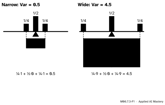
Measure how far each value sits from the mean \(\mu\). The signed distances \({x - \mu}\) cancel on average (that is what makes \(\mu\) the balance point), so they cannot measure spread. Square them instead: no square is negative, and far values count much more than near ones. A squared distance is a real square, side \({\abs{x - \mu}}\), so the spread becomes an average area.
M06.7.3-F1
Two PMFs that both balance at 3. Under each, a square for every value’s distance from the mean. The variance is the average area of the squares, weighted by probability: 0.5 on the left, 4.5 on the right.
That weighted average area is the variance. Its square root, the standard deviation, brings the answer back to the units of \(X\): here \({\sqrt{0.5} \approx 0.71}\) and \({\sqrt{4.5} \approx 2.12}\).
Build it up
Step 1. Deviations. For a die, \({\mu = 3.5}\) and the deviations \({x - 3.5}\) are \({-2.5, -1.5, -0.5, 0.5, 1.5, 2.5}\). Their average is 0.
Step 2. Square them and average. The squares are 6.25, 2.25, 0.25, 0.25, 2.25, 6.25, with total 17.5. Each has probability \(1/6\), so the variance is \({17.5/6 = 35/12 \approx 2.92}\).
Step 3. Back to the units of \(X\). If \(X\) is in pips, the variance is in squared pips. The standard deviation is \({\sqrt{35/12} \approx 1.71}\) pips: a typical distance from the mean.
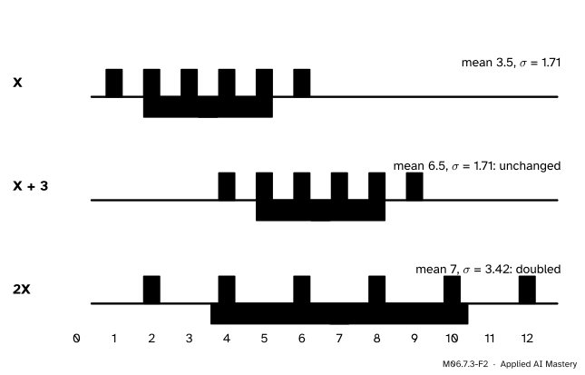
Step 4. Shift and stretch. Add 3 to every value and the whole picture slides right; no distance from the mean changes. Double every value and every distance doubles, so every square grows four times.
M06.7.3-F2
The orange band runs one standard deviation either side of the mean. A shift moves the band; a stretch by 2 doubles its width.
The formal statement
NoteDefinition: variance and standard deviation
For a random variable \(X\) with mean \({\mu = \E[X]}\), \[
\operatorname{Var}(X) = \E\big[(X - \mu)^2\big],
\]\[
\sigma_X = \sqrt{\operatorname{Var}(X)} .
\] For a PMF, \({\operatorname{Var}(X)}\)\({= \sum_x (x - \mu)^2\,p_X(x)}\); for a density, the same with an integral.
The shortcut. Expand the square and use linearity, remembering that \(\mu\) is a number:
The gap between the mean of the squares and the square of the mean, met in the last lesson, is the variance. Since a variance is an average of squares, it is never negative, and so \({\E[X^2] \ge (\E[X])^2}\) always.
Go deeper: why squares, and not distances without a sign?
The mean absolute deviation \({\E[\abs{X - \mu}]}\) also measures spread, and for the die it is \({(2.5 + 1.5 + 0.5) \cdot 2/6}\)\({= 1.5}\). Squares win for three reasons. They expand by algebra, which gives the shortcut above and the clean rules below; an absolute value does not. Variances of independent variables add, which standard deviations and mean absolute deviations do not. And squared error is the loss that the mean minimises (M06.7.4), so the variance is the smallest expected squared error a single guess can achieve. Machine learning meets the same choice as mean squared error against mean absolute error (ML01.4.1).
Shift and stretch. Let \({Y = aX + b}\). By linearity \({\E[Y] = a\mu + b}\), so the deviations of \(Y\) are \({Y - \E[Y]}\)\({= aX + b - a\mu - b}\)\({= a(X - \mu)}\). The shift \(b\) has cancelled. Then
and \({\sigma_{aX + b}}\)\({= \abs{a}\,\sigma_X}\).
Sums of independent variables. Let \(X\) and \(Y\) be independent, with means \(\mu_X\) and \(\mu_Y\). The deviation of the sum is \({(X - \mu_X) + (Y - \mu_Y)}\). Square it and take expectations:
The two deviations are independent too: \({X - \mu_X = u}\) is the same event as \({X = u + \mu_X}\), and likewise for \(Y\). So by the product rule of the last lesson the cross term is \({2\,\E[X - \mu_X]\,\E[Y - \mu_Y]}\)\({= 2 \cdot 0 \cdot 0}\)\({= 0}\). So for independent \(X\) and \(Y\),
Variances add; standard deviations do not. For dependent variables the cross term stays, and M06.10.2 names it: twice the covariance.
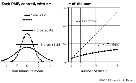
The square-root law. Add \(n\) independent copies of \(X\), each with variance \(\sigma^2\). The variances add to \({n\sigma^2}\), so the standard deviation of the sum is \({\sigma\sqrt{n}}\). Four times as many copies only doubles the spread, even though the range of possible totals grows four times.
M06.7.3-F3
The spread of a sum of \(n\) independent dice. Its standard deviation is \({1.71\sqrt{n}}\), not \({1.71\,n}\): 1.71, 3.42 and 6.83 for 1, 4 and 16 dice.
Worked example
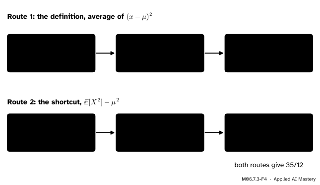
One die, both ways. By the definition, \({\operatorname{Var}(X)}\)\({= 17.5/6}\)\({= 35/12}\) (Build it up). By the shortcut, \({\E[X^2] = 91/6}\) (M06.7.1), so
The variance of one die by the definition (top) and by the shortcut (bottom). Both routes end at \({35/12 \approx 2.92}\).
A Bernoulli variable. If \(X\) is 1 with probability \(p\) and 0 otherwise, then \({X^2 = X}\), so \({\E[X^2] = p}\) and
\[
\operatorname{Var}(X) = p - p^2 = p(1 - p).
\]
A test example answered correctly with probability 0.9 has variance \({0.9 \times 0.1 = 0.09}\) and standard deviation 0.3. The number correct out of 100 independent examples then has variance \({100 \times 0.09 = 9}\) and standard deviation 3: about 90 correct, give or take 3.
The sum of two dice. The dice are independent, so \({\operatorname{Var}}\)\({= 35/12 + 35/12}\)\({= 35/6}\)\({\approx 5.83}\), and \({\sigma}\)\({= \sqrt{35/6}}\)\({\approx 2.42}\).
The hand density.\({\E[X^2]}\)\({= \int_0^1 x^2 \cdot 2x\,dx}\)\({= [x^4/2]_0^1}\)\({= 1/2}\), so
and \({\sigma}\)\({= \sqrt{1/18}}\)\({\approx 0.236}\).
Code
From scratch with exact fractions, by the definition and by the shortcut.
from fractions import Fractiondef mean(pmf):returnsum(x * p for x, p in pmf.items())def var(pmf): m = mean(pmf)returnsum((x - m) **2* p for x, p in pmf.items())def var_shortcut(pmf):returnsum(x * x * p for x, p in pmf.items()) - mean(pmf) **2die = {k: Fraction(1, 6) for k inrange(1, 7)}bern = {1: Fraction(9, 10), 0: Fraction(1, 10)}two_dice = {}for a inrange(1, 7):for b inrange(1, 7): two_dice[a + b] = two_dice.get(a + b, 0) + Fraction(1, 36)for name, pmf in [("die", die), ("Bernoulli(0.9)", bern), ("sum of two dice", two_dice)]:print(f"{name:16} Var = {var(pmf)} (shortcut {var_shortcut(pmf)}), sd = {float(var(pmf)) **0.5:.3f}")doubled = {2* x: p for x, p in die.items()}print("2X:", var(doubled), " X + 3:", var({x +3: p for x, p in die.items()}))
die              Var = 35/12  (shortcut 35/12),  sd = 1.708
Bernoulli(0.9)   Var = 9/100  (shortcut 9/100),  sd = 0.300
sum of two dice  Var = 35/6  (shortcut 35/6),  sd = 2.415
2X: 35/3    X + 3: 35/12
Now with simulated draws. numpy.var divides by the number of values \(N\) by default (ddof=0), which is the variance of the draws as a list; S02 explains when to divide by \({N - 1}\) instead.
import numpy as nprng = np.random.default_rng(2)rolls = rng.integers(1, 7, size=(16, 200_000)) # 16 independent dice, 200,000 timesprint("one die: var", rolls[0].var().round(3), " sd", rolls[0].std().round(3))for n in (1, 4, 16): totals = rolls[:n].sum(axis=0)print(f"sum of {n:2} dice: sd {totals.std():.2f} 1.71 * sqrt(n) = {np.sqrt(35/12* n):.2f}")hand = np.sqrt(rng.random(200_000)) # draws from the density 2xprint("density 2x: var", hand.var().round(4), " exact 1/18 =", round(1/18, 4))
one die:   var 2.921   sd 1.709
sum of  1 dice: sd 1.71   1.71 * sqrt(n) = 1.71
sum of  4 dice: sd 3.42   1.71 * sqrt(n) = 3.42
sum of 16 dice: sd 6.83   1.71 * sqrt(n) = 6.83
density 2x: var 0.0558   exact 1/18 = 0.0556
Explore
M06.7-X1
Balance beam
Raise or lower any bar (drag it, or pick a value and use the slider) and the others rescale to keep the total 1: watch the pivot, at the mean, and the band, one standard deviation either side. Then try the shift and stretch buttons, and check that the band ignores \(b\) but scales with \(a\).
Things to try. Put all the weight on the two ends (“Two ends”): the variance is as large as it can be on 0 to 6, 9. Pile it on one value: the band vanishes. Move weight next to the pivot and the band hardly moves; move the same weight to an end and it widens a lot, because distances are squared.
Pitfalls
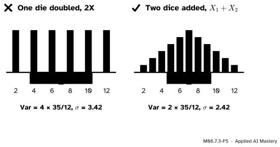
M06.7.3-F5
Wrong beside right. Treating the sum of two dice as one die doubled gives the wrong spread: the true sum is a triangle, with variance \({2 \times 35/12}\), not \({4 \times 35/12}\).
“Two dice are just one die counted twice: Var(X₁ + X₂) = Var(2X).”
The means agree (7 both ways), but the spreads do not. Doubling one die keeps every outcome extreme: a 6 becomes 12. Two independent dice tend to offset each other, so the total gathers near 7. Variance \({4 \times 35/12}\) for \({2X}\), \({2 \times 35/12}\) for \({X_1 + X_2}\). This is why averaging independent measurements reduces noise, and why a mini-batch gradient is less noisy than a single-example one.
“Standard deviations add.”
Variances of independent variables add; standard deviations do not. For two dice \({\sigma}\)\({= \sqrt{35/6}}\)\({\approx 2.42}\), not \({1.71 + 1.71 = 3.42}\). Add the squares, then take the root, as with the sides of a right triangle.
“Var(X − Y) = Var(X) − Var(Y).”
For independent \(X\) and \(Y\), \({X - Y = X + (-1)Y}\), and the stretch by \(-1\) multiplies the variance of \(Y\) by \({(-1)^2 = 1}\), so the variances still add. Subtracting a noisy quantity adds its noise. Variances can never be negative, and \({\operatorname{Var}(X) - \operatorname{Var}(Y)}\) could be.
Check yourself
Recall
1. Define the variance and the standard deviation of \(X\).
Show answer
\({\operatorname{Var}(X)}\)\({= \E[(X - \mu)^2]}\), the expected squared distance from the mean; \({\sigma_X}\)\({= \sqrt{\operatorname{Var}(X)}}\), in the units of \(X\).
3. What are \({\operatorname{Var}(aX + b)}\) and \({\sigma_{aX + b}}\)?
Show answer
\({a^2 \operatorname{Var}(X)}\) and \({\abs{a}\,\sigma_X}\). The shift \(b\) changes neither.
4. What is the variance of a Bernoulli(\(p\)) variable?
Show answer
\({p(1 - p)}\), because \({\E[X^2] = \E[X] = p}\).
5. How does the standard deviation of a sum of \(n\) independent copies grow with \(n\)?
Show answer
Like \({\sqrt{n}}\): the variances add to \({n\sigma^2}\), so the standard deviation is \({\sigma\sqrt{n}}\).
Exercises
1.★ For a die roll \(X\), find the variance and standard deviation of the payout \({2X - 5}\).
Show solution
\({\operatorname{Var}(2X - 5)}\)\({= 4 \times 35/12}\)\({= 35/3}\)\({\approx 11.67}\), and the standard deviation is \({2 \times 1.71 = 3.42}\) pounds. The \(-5\) changes the mean, not the spread.
2.★★ Find the variance of \({U \sim \text{Unif}(0, 1)}\), and use it to find the variance of \({\text{Unif}(a, b)}\).
Show solution
\({\E[U] = 1/2}\) and \({\E[U^2]}\)\({= \int_0^1 u^2\,du}\)\({= 1/3}\), so \({\operatorname{Var}(U)}\)\({= 1/3 - 1/4}\)\({= 1/12}\). A uniform on \([a, b]\) is \({a + (b - a)U}\), a shift and a stretch by \({b - a}\), so its variance is \({(b - a)^2/12}\).
3.★★★ Two independent dice are rolled and \(D\) is the first minus the second. Find \({\E[D]}\) and \({\operatorname{Var}(D)}\), and check the variance by listing the PMF of \(D\).
Show solution
\({\E[D] = 3.5 - 3.5 = 0}\), and \({\operatorname{Var}(D)}\)\({= 35/12 + (-1)^2 \cdot 35/12}\)\({= 35/6}\). The PMF of \(D\) is \({\Prob(D = d)}\)\({= (6 - \abs{d})/36}\) for \({d = -5, \dots, 5}\). Since \({\E[D] = 0}\), the variance is \({\E[D^2]}\):
Independent:\({\operatorname{Var}(X + Y)}\)\({= \operatorname{Var}(X) + \operatorname{Var}(Y)}\); \(n\) copies have \({\sigma\sqrt{n}}\).
Values: die \({35/12}\); Bernoulli \({p(1 - p)}\); two dice \({35/6}\); density \({2x}\): \({1/18}\).
Sources and next steps
Sources. Each was opened and checked against this lesson on 12 November 2026.
Charles M. Grinstead and J. Laurie Snell, Introduction to Probability, second edition, Section 6.2: Definition 6.3 (variance and standard deviation), Example 6.17 (one die, \({V(X) = 35/12}\), \({D(X) \approx 1.707}\)), Theorem 6.6 (the shortcut), Theorem 6.7 (\({V(cX) = c^2 V(X)}\) and \({V(X + c) = V(X)}\)), Theorem 6.8 (variances of independent variables add) and Theorem 6.9 (a sum of \(n\) has variance \({n\sigma^2}\)).
Jeremy Orloff and Jonathan Bloom, Reading 5a: Variance of Discrete Random Variables, MIT OpenCourseWare 18.05, Spring 2022. Section 3 reads the variance as a weighted average of squared distances and notes the units of \(\sigma\) and of the variance; Section 3.1 derives \({p(1 - p)}\) for a Bernoulli variable.
Hossein Pishro-Nik, Variance, Section 3.2.4 (Equations 3.5 to 3.7, with the die worked to about 2.92), and Expected Value and Variance, Section 4.1.2, the variance of a continuous variable, in Introduction to Probability, Statistics, and Random Processes.
NumPy, numpy.var: the divisor is \({N - \text{ddof}}\), with ddof=0 by default.
Next.M06.7.4 Standardising and higher moments uses the mean and standard deviation to put any variable on a common scale, and reads its shape from the third and fourth moments.